Chapter 1: Vectors
I’m committing crimes with both direction and magnitude.
—Vector, Despicable Me


The stick chart is a navigational tool crafted by the indigenous people of the Marshall Islands, located in the central Pacific Ocean. This ancient tool was made by carefully tying together the midribs of coconut fronds. Shell markings on the chart signify the locations of islands in the region. The layout of the fronds and shells serves as a geographical guide, offering an abstract representation of vectors that capture the ocean swell patterns and their directional flow.
This book is all about looking at the world around us and developing ways to simulate it with code. In this first part of the book, I’ll start by looking at basic physics: how an apple falls from a tree, how a pendulum swings in the air, how Earth revolves around the sun, and so on. Absolutely everything contained within the book’s first five chapters requires the use of the most basic building block for programming motion, the vector. And so that’s where I’ll begin the story.
The word vector can mean a lot of things. It’s the name of a New Wave rock band formed in Sacramento, California, in the early 1980s, and the name of a breakfast cereal manufactured by Kellogg’s Canada. In the field of epidemiology, a vector is an organism that transmits infection from one host to another. In the C++ programming language, a vector (std::vector) is an implementation of a dynamically resizable array data structure.
While all these definitions are worth exploring, they’re not the focus here. Instead, this chapter dives into the Euclidean vector (named for the Greek mathematician Euclid), also known as the geometric vector. When you see the term vector in this book, you can assume it refers to a Euclidean vector, defined as an entity that has both magnitude and direction.


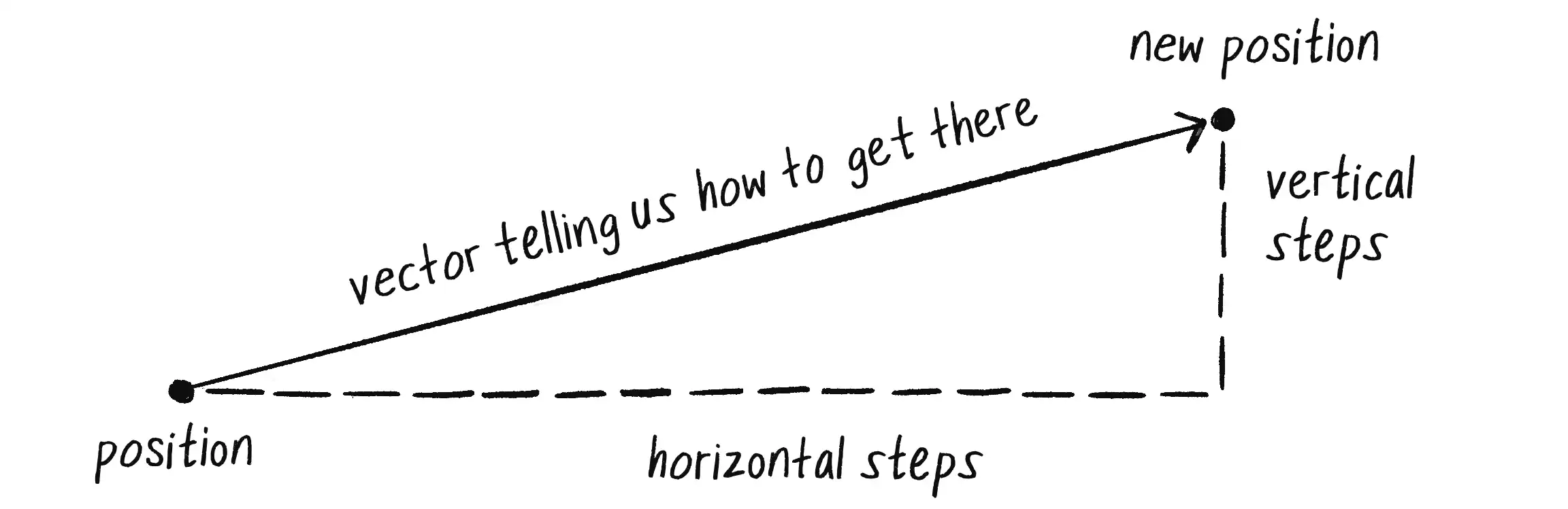
A vector is typically drawn as an arrow, as in Figure 1.1. The vector’s direction is indicated by where the arrow is pointing, and its magnitude by the length of the arrow.
The vector in Figure 1.1 is drawn as an arrow from point A to point B. It serves as an instruction for how to travel from A to B.
The Point of Vectors

Before diving into more details about vectors, I’d like to create a p5.js example that demonstrates why you should care about vectors in the first place. If you’ve watched any beginner p5.js tutorials, read any introductory p5.js textbooks, or taken an introduction to creative coding course (and hopefully you’ve done one of these things to help prepare you for this book!), you probably, at one point or another, learned how to write a bouncing ball sketch.
Example 1.1: Bouncing Ball with No Vectors
let x = 100;
let y = 100;
let xspeed = 2.5;
let yspeed = 2;
function setup() {
createCanvas(640, 240);
}
function draw() {
background(255);
  x = x + xspeed;
  y = y + yspeed;
Move the ball according to its speed.
  if (x > width || x < 0) {
    xspeed = xspeed * -1;
  }
  if (y > height || y < 0) {
    yspeed = yspeed * -1;
  }
Check for bouncing.
  stroke(0);
  fill(127);
  circle(x, y, 48);
Draw the ball at the position (x, y).
}
In this example, there’s a flat, 2D world—a blank canvas—with a circular shape (a “ball”) traveling around. This ball has properties like position and speed that are represented in the code as variables:
| Property | Variable Names |
|---|---|
| Position | x and y |
| Speed | xspeed and yspeed |
In a more sophisticated sketch, you might have many more variables representing other properties of the ball and its environment:
| Property | Variable Names |
|---|---|
| Acceleration | xacceleration and yacceleration |
| Target position | xtarget and ytarget |
| Wind | xwind and ywind |
| Friction | xfriction and yfriction |
You might notice that for every concept in this world (wind, position, acceleration, and the like), there are two variables. And this is only a 2D world. In a three-dimensional (3D) world, you’d need three variables for each property: x, y, and z for position; xspeed, yspeed, and zspeed for speed; and so on. Wouldn’t it be nice to simplify the code to use fewer variables? Instead of starting the program with something like this
let x;
let y;
let xspeed;
let yspeed;
you’d be able to start it with something like this:
let position;
let speed;
Thinking of the ball’s properties as vectors instead of a loose collection of separate values will allow you to do just that.
Taking this first step toward using vectors won’t let you do anything new or magically turn a p5.js sketch into a full-on physics simulation. However, using vectors will help organize your code and provide a set of methods for common mathematical operations you’ll need over and over and over again while programming motion.
As an introduction to vectors, I’m going to stick to two dimensions for quite some time (at least the first several chapters). All these examples can be fairly easily extended to three dimensions (and the class I’ll use, p5.Vector, allows for three dimensions). However, for the purposes of learning the fundamentals, the added complexity of the third dimension would be a distraction.
Vectors in p5.js
Think of a vector as the difference between two points, or as instructions for walking from one point to another. For example, Figure 1.2 shows some vectors and possible interpretations of them.

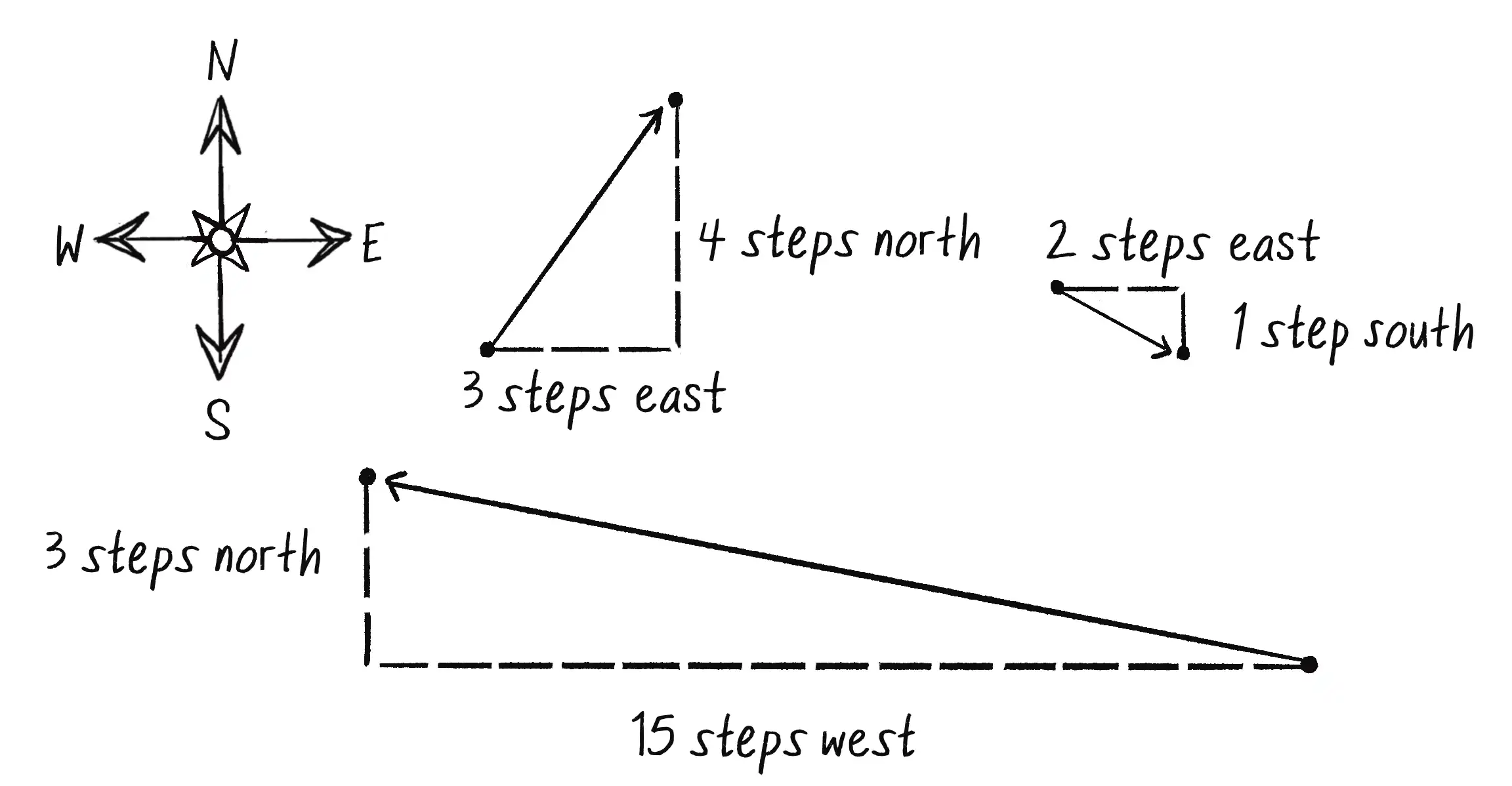
These vectors could be thought of in the following way:
| Vector | Instructions |
|---|---|
| (–15, 3) | Walk 15 steps west; turn and walk 3 steps north. |
| (3, 4) | Walk 3 steps east; turn and walk 4 steps north. |
| (2, –1) | Walk 2 steps east; turn and walk 1 step south. |
You’ve probably already thought this way when programming motion. For every frame of animation (a single cycle through a p5.js draw() loop), you instruct each object to reposition itself to a new spot a certain number of pixels away horizontally and a certain number of pixels away vertically. This instruction is essentially a vector, as in Figure 1.3; it has both magnitude (how far away did you travel?) and direction (which way did you go?).

The vector sets the object’s velocity, defined as the rate of change of the object’s position with respect to time. In other words, the velocity vector determines the object’s new position for every frame of the animation, according to this basic algorithm for motion: the new position is equal to the result of applying the velocity to the current position.
If velocity is a vector (the difference between two points), what about position? Is it a vector too? Technically, you could argue that position is not a vector, since it’s not describing how to move from one point to another; it’s describing a single point in space. Nevertheless, another way to describe a position is as the path taken from the origin—point (0, 0)—to the current point. When you think of position in this way, it becomes a vector, just like velocity, as in Figure 1.4.


In Figure 1.4, the vectors are placed on a computer graphics canvas. Unlike in Figure 1.2, the origin point (0, 0) isn’t at the center; it’s at the top-left corner. And instead of north, south, east, and west, there are positive and negative directions along the x- and y-axes (with y pointing down in the positive direction).
Let’s examine the underlying data for both position and velocity. In the bouncing ball example, I originally had the following variables:
| Property | Variable Names |
|---|---|
| Position | x, y |
| Velocity | xspeed, yspeed |
Now I’ll treat position and velocity as vectors instead, each represented by an object with x and y attributes. If I were to write a Vector class myself, I’d start with something like this:
class Vector {
constructor(x, y) {
this.x = x;
this.y = y;
}
}
Notice that this class is designed to store the same data as before—two floating-point numbers per vector, an x value and a y value. At its core, a Vector object is just a convenient way to store two values (or three, as you’ll see in 3D examples) under one name.
As it happens, p5.js already has a built-in p5.Vector class, so I don’t need to write one myself. And so this
let x = 100;
let y = 100;
let xspeed = 1;
let yspeed = 3.3;
becomes this:
let position = createVector(100, 100);
let velocity = createVector(1, 3.3);
Notice that the position and velocity vector objects aren’t created as you might expect, by invoking a constructor function. Instead of writing new p5.Vector(x, y), I’ve called createVector(x, y). The createVector() function is included in p5.js as a helper function to take care of details behind the scenes upon creation of the vector. Except in special circumstances, you should always create p5.Vector objects with createVector(). I should note that p5.js functions such as createVector() can’t be executed outside of setup() or draw(), since the library won’t yet be loaded. I’ll demonstrate how to address this in Example 1.2.
Now that I have two vector objects (position and velocity), I’m ready to implement the vector-based algorithm for motion: position = position + velocity. In Example 1.1, without vectors, the code reads as follows:
x = x + xspeed;
y = y + yspeed;
Add each speed to each position.
In an ideal world, I would be able to rewrite this as shown here:
position = position + velocity;
Add the velocity vector to the position vector.
In JavaScript, however, the addition operator + is reserved for primitive values (integers, floats, and the like). JavaScript doesn’t know how to add two p5.Vector objects together any more than it knows how to add two p5.Font objects or p5.Image objects. Fortunately, the p5.Vector class includes methods for common mathematical operations.
Vector Addition

Before I continue working with the p5.Vector class and the add() method, let’s examine vector addition by using the notation found in math and physics textbooks. Vectors are typically written either in boldface type or with an arrow on top. For the purposes of this book, to distinguish a vector (with magnitude and direction) from a scalar (a single value, such as an integer or a floating-point number), I’ll use the arrow notation:
- Vector:
- Scalar:
Let’s say I have the two vectors shown in Figure 1.5.


Each vector has two components, an x and a y. To add the two vectors together, add both x-components and y-components to create a new vector, as in Figure 1.6.

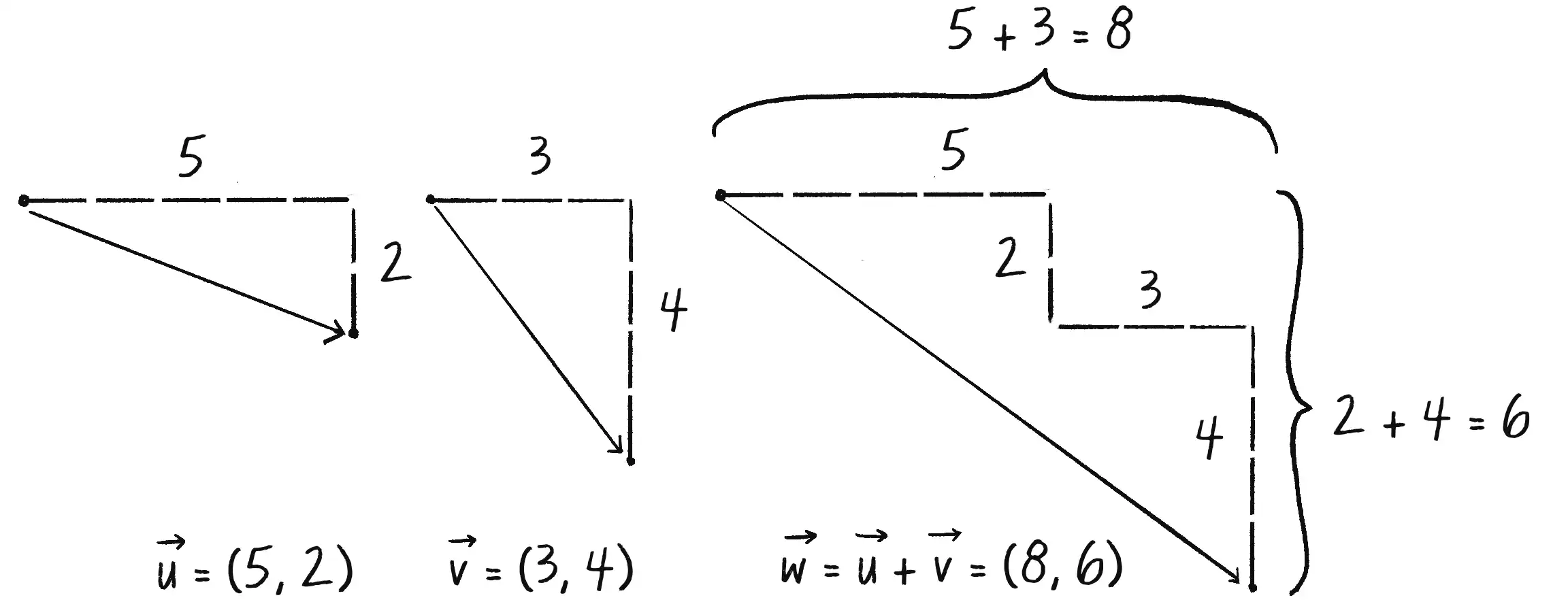
In other words, can be written as follows:
Then, replacing and with their values from Figure 1.6, you get this:
Finally, write the result as a vector:
Addition Properties with Vectors
Addition with vectors follows the same algebraic rules as with real numbers.
The commutative rule:
The associative rule:
Fancy terminology and symbols aside, these rules boil down to quite a simple concept: the result is the same no matter the order in which the vectors are added. Replace the vectors with regular numbers (scalars), and these rules are easy to see:
Commutative:
Associative:
Now that I’ve covered the theory behind adding two vectors together, I can turn to adding vector objects in p5.js. Imagine again that I’m creating my own Vector class. I could give it a function called add() that takes another Vector object as its argument:
class Vector {
constructor(x, y) {
this.x = x;
this.y = y;
}
  add(v) {
    this.x = this.x + v.x;
    this.y = this.y + v.y;
  }
New! A function to add another vector to this vector. Add the x-components and the y-components separately.
}
The function looks up the x- and y-components of the two vectors and adds them separately. This is exactly how the built-in p5.Vector class’s add() method is written too. Knowing how it works, I can now return to the bouncing ball example with its position + velocity algorithm and implement vector addition:
position = position + velocity;
This does not work!
position.add(velocity);
Add the velocity to the position.
Now you have what you need to rewrite the bouncing ball example with vectors.
Example 1.2: Bouncing Ball with Vectors!
let position;
let velocity;
Instead of a bunch of floats, you now have just two variables.
function setup() {
createCanvas(640, 240);
  position = createVector(100, 100);
  velocity = createVector(2.5, 2);
Note that createVector() has to be called inside setup().
}
function draw() {
background(255);
position.add(velocity);
  if (position.x > width || position.x < 0) {
    velocity.x = velocity.x * -1;
  }
  if (position.y > height || position.y < 0) {
    velocity.y = velocity.y * -1;
  }
You still sometimes need to refer to the individual components of a p5.Vector and can do so using the dot syntax: position.x, velocity.y, and so forth.
stroke(0);
fill(127);
circle(position.x, position.y, 48);
}
At this stage, you might feel somewhat disappointed. After all, these changes may appear to have made the code more complicated than the original version. While this is a perfectly reasonable and valid critique, it’s important to understand that the power of programming with vectors hasn’t been fully realized just yet. Looking at a bouncing ball and only implementing vector addition is just the first step. As I move forward into a more complex world of multiple objects and multiple forces (which I’ll introduce in Chapter 2) acting on those objects, the benefits of vectors will become more apparent.
I should, however, note an important aspect of the transition to programming with vectors. Even though I’m using p5.Vector objects to encapsulate two values—the x and y of the ball’s position or the x and y of the ball’s velocity—under a single variable name, I’ll still often need to refer to the x- and y-components of each vector individually.
The circle() function doesn’t allow for a p5.Vector object as an argument. A circle can be drawn with only two scalar values, an x-coordinate and a y-coordinate. And so I must dig into the p5.Vector object and pull out the x- and y-components by using object-oriented dot syntax:
circle(position, 48);
circle(position.x, position.y, 48);
The same issue arises when testing whether the circle has reached the edge of the window. In this case, I need to access the individual components of both vectors, position and velocity:
if ((position.x > width) || (position.x < 0)) {
velocity.x = velocity.x * -1;
}
It may not always be obvious when to directly access an object’s properties versus when to reference the object as a whole or use one of its methods. The goal of this chapter (and most of this book) is to help you distinguish between these scenarios by providing a variety of examples and use cases.
Exercise 1.1
Take one of the walker examples from Chapter 0 and convert it to use vectors.
Exercise 1.2
Find something else you’ve previously made in p5.js using separate x and y variables, and use vectors instead.
Exercise 1.3
Extend Example 1.2 into 3D. Can you get a sphere to bounce around a box?
More Vector Math
Addition was really just the first step. Many mathematical operations are commonly used with vectors. Here’s a comprehensive table of the operations available as methods in the p5.Vector class. Remember, these are not stand-alone functions, but rather methods associated with the p5.Vector class. When you see the word this in the following table, it refers to the specific vector the method is operating on.
| Method | Task |
|---|---|
| Adds a vector to this vector |
| Subtracts a vector from this vector |
| Scales this vector with multiplication |
| Scales this vector with division |
| Returns the magnitude of this vector |
| Sets the magnitude of this vector |
| Normalizes this vector to a unit length of 1 |
| Limits the magnitude of this vector |
| Returns the 2D heading of this vector expressed as an angle |
| Rotates this 2D vector by an angle |
| Linear interpolates to another vector |
| Returns the Euclidean distance between two vectors (considered as points) |
| Finds the angle between two vectors |
| Returns the dot product of two vectors |
| Returns the cross product of two vectors (relevant only in three dimensions) |
| Returns a random 2D vector |
| Returns a random 3D vector |
I’ll go through a few of the key methods now. As the examples get more sophisticated in later chapters, I’ll continue to reveal more details.
Vector Subtraction


Having already covered addition, I’ll now turn to subtraction. This one’s not so bad; just take the plus sign and replace it with a minus! Before tackling subtraction itself, however, consider what it means for a vector to become . The negative version of the scalar 3 is –3. A negative vector is similar: the polarity of each of the vector’s components is inverted. So if has the components (x, y), then is (–x, –y). Visually, this results in an arrow of the same length as the original vector pointing in the opposite direction, as depicted in Figure 1.7.
Subtraction, then, is the same as addition, only with the second vector in the equation treated as a negative version of itself:
Just as vectors are added by placing them “tip to tail”—that is, aligning the tip (or endpoint) of one vector with the tail (or start point) of the next—vectors are subtracted by reversing the direction of the second vector and placing it at the end of the first, as in Figure 1.8.

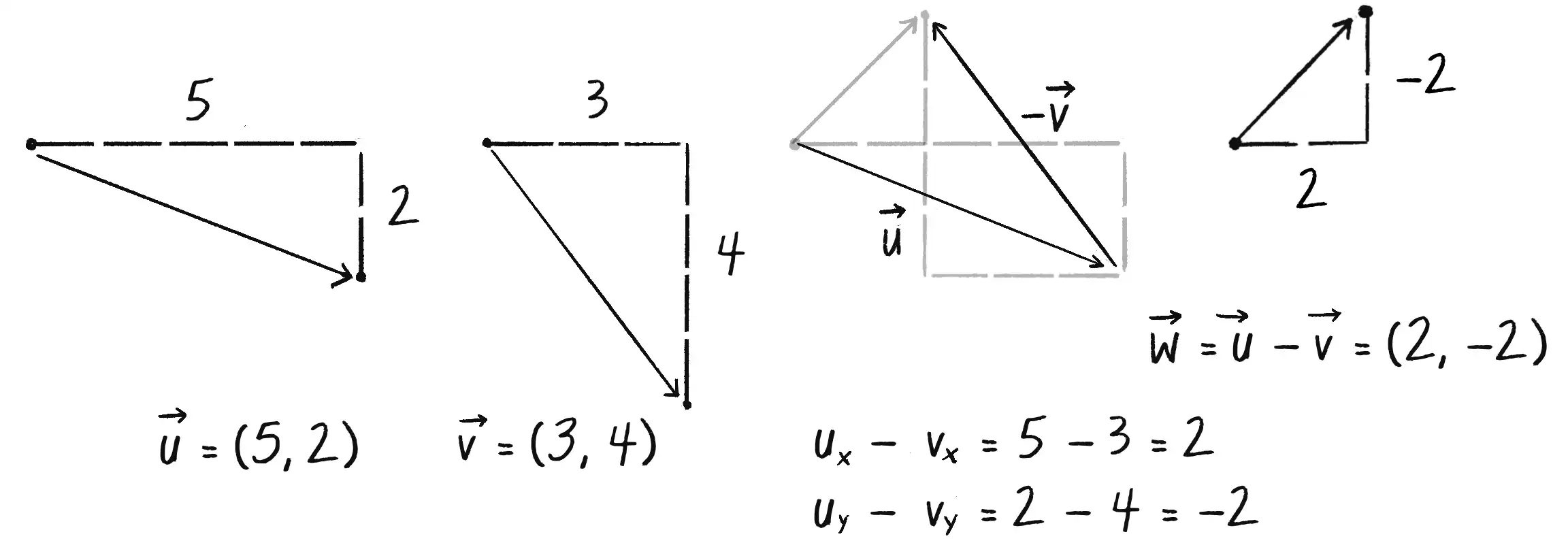
To actually solve the subtraction, take the difference of the vectors’ components. That is, can be written as shown here:
Inside p5.Vector, the code reads as follows:
sub(v) {
this.x = this.x - v.x;
this.y = this.y - v.y;
}
The following example demonstrates vector subtraction by taking the difference between two points (which are treated as vectors): the mouse position and the center of the window.
Example 1.3: Vector Subtraction
function draw() {
background(255);
  let mouse = createVector(mouseX, mouseY);
  let center = createVector(width / 2, height / 2);
Two vectors, one for the mouse location and one for the center of the window
  stroke(200);
  strokeWeight(4);
  line(0, 0, mouse.x, mouse.y);
  line(0, 0, center.x, center.y);
Draw the original two vectors.
mouse.sub(center);
Vector subtraction!
  stroke(0);
  translate(width / 2, height / 2);
  line(0, 0, mouse.x, mouse.y);
Draw a line to represent the result of subtraction.
Notice that I move the origin with translate() to place the vector.
}
Note the use of translate() to visualize the resulting vector as a line from the center (width / 2, height / 2) to the mouse. Vector subtraction is its own kind of translation, moving the “origin” of a position vector. Here, by subtracting the center vector from the mouse vector, I’m effectively moving the starting point of the resulting vector to the center of the canvas. Therefore, I also need to move the origin by using translate(). Without this, the line would be drawn from the top-left corner, and the visual connection wouldn’t be as clear.
Vector Multiplication and Division

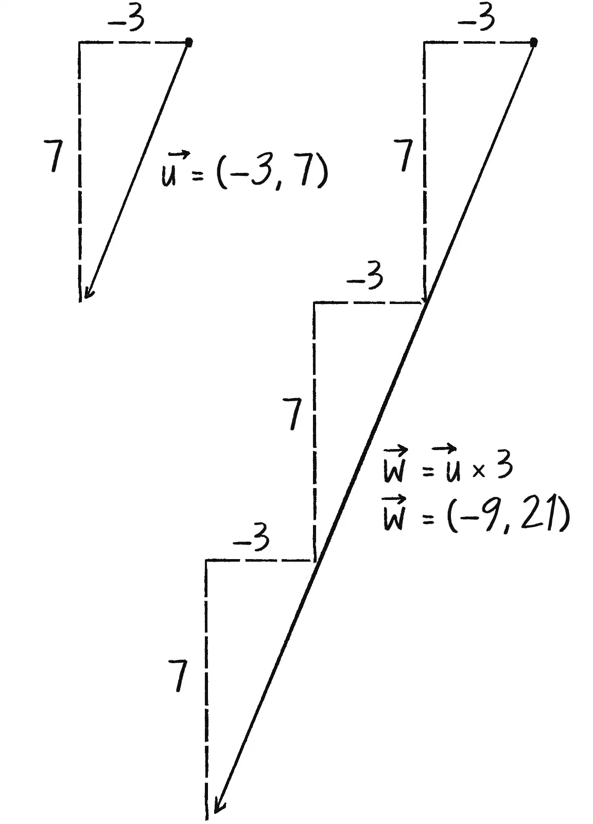
Moving on to multiplication, you have to think a bit differently. Multiplying a vector typically refers to the process of scaling a vector. If I want to scale a vector to twice its size or one-third of its size, while leaving its direction the same, I would say, “Multiply the vector by 2” or “Multiply the vector by 1/3.” Unlike with addition and subtraction, I’m multiplying the vector by a scalar (a single number), not by another vector. Figure 1.9 illustrates how to scale a vector by a factor of 3.
To scale a vector, multiply each component (x and y) by a scalar. That is, can be written as shown here:
As an example, say and . You can calculate as follows:
This is exactly how the mult() function inside the p5.Vector class works:
mult(n) {
  this.x = this.x * n;
  this.y = this.y * n;
The components of the vector are multiplied by a number.
}
Implementing multiplication in code is as simple as the following:
let u = createVector(-3, 7);
u.mult(3);
This p5.Vector is now three times the size and is equal to (–9, 21). See Figure 1.9.
Example 1.4 illustrates vector multiplication by drawing a line between the mouse and the center of the canvas, as in the previous example, and then scaling that line by 0.5.
Example 1.4: Multiplying a Vector
function draw() {
background(255);
let mouse = createVector(mouseX, mouseY);
let center = createVector(width / 2, height / 2);
mouse.sub(center);
translate(width / 2, height / 2);
strokeWeight(2);
stroke(200);
line(0, 0, mouse.x, mouse.y);
mouse.mult(0.5);
Multiplying a vector! The vector is now half its original size (multiplied by 0.5).
stroke(0);
strokeWeight(4);
line(0, 0, mouse.x, mouse.y);
}
The resulting vector is half its original size. Rather than multiplying the vector by 0.5, I could achieve the same effect by dividing the vector by 2, as in Figure 1.10.


Vector division, then, works just like vector multiplication—just replace the multiplication sign (*) with the division sign (/). Here’s how the p5.Vector class implements the div() function:
div(n) {
this.x = this.x / n;
this.y = this.y / n;
}
And here’s how to use the div() function in a sketch:
let u = createVector(8, -4);
u.div(2);
Dividing a vector! The vector is now half its original size (divided by 2).
This takes the vector u and divides it by 2.
More Number Properties with Vectors
As with addition, basic algebraic rules of multiplication apply to vectors.
The associative rule:
The distributive rule with two scalars, one vector:
The distributive rule with two vectors, one scalar:
Vector Magnitude


Multiplication and division, as just described, alter the length of a vector without affecting its direction. Perhaps you’re wondering, “Okay, so how do I know what the length of a vector is? I know the vector’s components (x and y), but how long (in pixels) is the actual arrow?” Understanding how to calculate the length of a vector, also known as its magnitude, is incredibly useful and important.


Notice in Figure 1.11 that the vector, drawn as an arrow and two components (x and y), creates a right triangle. The sides are the components, and the hypotenuse is the arrow. We’re lucky to have this right triangle, because once upon a time, a Greek mathematician named Pythagoras discovered a lovely formula that describes the relationship between the sides and hypotenuse of a right triangle. This formula, the Pythagorean theorem, is (see Figure 1.12).
Armed with this formula, we can now compute the magnitude of as follows:
In the p5.Vector class, the mag() function is defined using the same formula:
mag() {
return sqrt(this.x * this.x + this.y * this.y);
}
The sketch in the next example calculates the magnitude of the vector between the mouse and the center of the canvas, and visualizes it as a rectangle drawn across the top of the window.
Example 1.5: Vector Magnitude
function setup() {
createCanvas(640, 240);
}
function draw() {
background(255);
let mouse = createVector(mouseX, mouseY);
let center = createVector(width / 2, height / 2);
mouse.sub(center);
  let m = mouse.mag();
  fill(0);
  rect(0, 0, m, 10);
The magnitude (that is, length) of a vector can be accessed via the mag() method. Here it is used as the width of a rectangle drawn at the top of the window.
translate(width / 2, height / 2);
line(0, 0, mouse.x, mouse.y);
}
Notice that the magnitude (length) of a vector is always positive, even if the vector’s components are negative.
Normalizing Vectors


Calculating the magnitude of a vector is only the beginning. It opens the door to many possibilities, the first of which is normalization (Figure 1.13). This is the process of making something standard or, well . . . normal. In the case of vectors, the convention is that a standard vector has a length of 1. To normalize a vector, therefore, is to take a vector of any length and change its length to 1, without changing its direction. That normalized vector is then called a unit vector.
A unit vector describes a vector’s direction without regard to its length. You’ll see this come in especially handy once you start to work with forces in Chapter 2.
For any given vector , its unit vector (written as ) is calculated as follows:

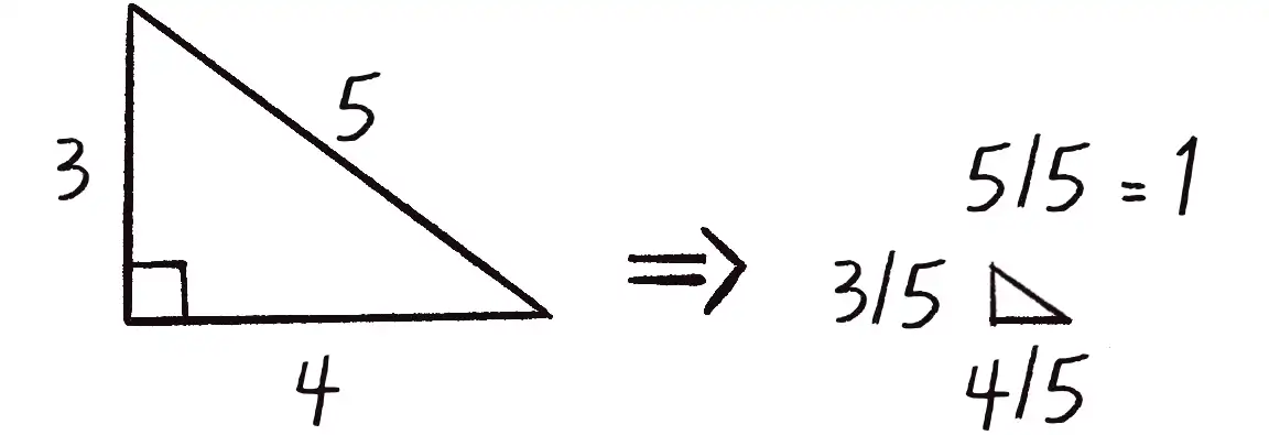
In other words, to normalize a vector, divide each component by the vector’s magnitude. To see why this works, consider a vector (4, 3), which has a magnitude of 5 (see Figure 1.14). Once normalized, the vector will have a magnitude of 1. Thinking of the vector as a right triangle, normalization shrinks the hypotenuse by dividing by 5 (since 5/5 = 1). In that process, each side shrinks as well, also by a factor of 5. The side lengths go from 4 and 3 to 4/5 and 3/5, respectively.
In the p5.Vector class, the normalization method is written as follows:
normalize() {
let m = this.mag();
this.div(m);
}
Of course, there’s one small issue. What if the magnitude of the vector is 0? You can’t divide by 0! Some quick error checking, shown next, fixes that right up.
normalize() {
let m = this.mag();
if (m > 0) {
this.div(m);
}
}
This sketch uses normalization to give the vector between the mouse and the center of the canvas a fixed length, regardless of the actual magnitude of the original vector.
Example 1.6: Normalizing a Vector
function draw() {
background(255);
let mouse = createVector(mouseX, mouseY);
let center = createVector(width / 2, height / 2);
mouse.sub(center);
translate(width / 2, height / 2);
stroke(200);
line(0, 0, mouse.x, mouse.y);
  mouse.normalize();
  mouse.mult(50);
In this example, after the vector is normalized, it’s multiplied by 50. Note that no matter where the mouse is, the vector always has the same length (50) because of the normalization process.
stroke(0);
strokeWeight(8);
line(0, 0, mouse.x, mouse.y);
}
Notice that I’ve multiplied the mouse vector by 50 after normalizing it to 1. Normalization is often the first step in creating a vector of a specific length, even if the desired length is something other than 1. You’ll see more of this later in the chapter.
All this vector math stuff sounds like something you should know about, but why? How will it help you write code? Patience. It’ll take some time before the awesomeness of using p5.Vector fully comes to light. This is a fairly common occurrence when learning a new data structure. For example, when you first learn about arrays, it might seem like more work to use an array than to have several variables stand for multiple things. That plan quickly breaks down when you need 100, 1,000, or 10,000 things, however.
The same can be true for vectors. What might seem like more work now will pay off later, and quite nicely. And you don’t have to wait too long, as your reward will come in the next chapter. For now, however, I’ll focus on how vectors work, and on how working with them provides a different way to think about motion.
Motion with Vectors
What does it mean to program motion by using vectors? You got a taste of it in Example 1.2, the bouncing ball. The circle onscreen has a position (its location at any given moment) as well as a velocity (instructions for how it should move from one moment to the next). Velocity is added to position:
position.add(velocity);
Then the object is drawn at the new position:
circle(position.x, position.y, 48);
Together, these steps are Motion 101:
- Add the velocity to the position.
- Draw the object at the position.
In the bouncing ball example, all this code happened within setup() and draw(). What I want to do now is move toward encapsulating all the logic for an object’s motion inside a class. This way, I can create a foundation for programming moving objects that I can easily reuse again and again. (See “The Random Walker Class” for a brief review of OOP basics.)
To start, I’m going to create a generic Mover class that will describe a shape moving around the canvas. For that, I must consider the following two questions:
- What data does a mover have?
- What functionality does a mover have?
The Motion 101 algorithm answers both of these questions. First, a Mover object has two pieces of data, position and velocity, which are both p5.Vector objects. These are initialized in the object’s constructor. In this case, I’ll arbitrarily decide to initialize the Mover object by giving it a random position and velocity. Note the use of this with all variables that are part of the Mover object:
class Mover {
constructor() {
this.position = createVector(random(width), random(height));
this.velocity = createVector(random(-2,2), random(-2, 2));
}
The functionality follows suit. The Mover object needs to move (by applying its velocity to its position) and needs to be visible. I’ll implement these needs as functions named update() and show(). I’ll put all the motion logic code in update() and draw the object in show():
update() {
this.position.add(this.velocity);
The mover moves.
}
show() {
stroke(0);
fill(175);
circle(this.position.x, this.position.y, 48);
The mover is drawn as a circle.
}
The Mover class also needs a function that determines what the object should do when it reaches the edge of the canvas. For now, I’ll do something simple and have it wrap around the edges:
checkEdges() {
    if (this.position.x > width) {
      this.position.x = 0;
    } else if (this.position.x < 0) {
      this.position.x = width;
    }

    if (this.position.y > height) {
      this.position.y = 0;
    } else if (this.position.y < 0) {
      this.position.y = height;
    }
When it reaches one edge, set the position to the other edge.
}
}
Now the Mover class is finished, but the class itself isn’t an object; it’s a template for creating an instance of an object. To actually create a Mover object, I first need to declare a variable to hold it:
let mover;
Then, inside the setup() function, I create the object by invoking the class name along with the new keyword. This triggers the class’s constructor to make an instance of the object:
mover = new Mover();
Now all that remains is to call the appropriate methods in draw():
  mover.update();
  mover.checkEdges();
  mover.show();
Here’s the entire example for reference.
Example 1.7: Motion 101 (Velocity)
let mover;
Declare the Mover object.
function setup() {
createCanvas(640, 240);
mover = new Mover();
Create the Mover object.
}
function draw() {
background(255);
mover.update();
mover.checkEdges();
mover.show();
Call methods on the Mover object.
}
class Mover {
constructor() {
    this.position = createVector(random(width), random(height));
    this.velocity = createVector(random(-2, 2), random(-2, 2));
The object has two vectors: position and velocity.
}
update() {
this.position.add(this.velocity);
Motion 101: position changes by velocity.
}
show() {
stroke(0);
strokeWeight(2);
fill(127);
circle(this.position.x, this.position.y, 48);
}
checkEdges() {
if (this.position.x > width) {
this.position.x = 0;
} else if (this.position.x < 0) {
this.position.x = width;
}
if (this.position.y > height) {
this.position.y = 0;
} else if (this.position.y < 0) {
this.position.y = height;
}
}
}
If OOP is at all new to you, one aspect here may seem a bit strange. I spent the beginning of this chapter discussing the p5.Vector class, and this class is the template for making the position object and the velocity object. So what are those objects doing inside yet another object, the Mover object?
In fact, this is just about the most normal thing ever. An object is something that holds data (and functionality). That data can be numbers, or it can be other objects (arrays too)! You’ll see this over and over again in this book. In Chapter 4, for example, I’ll write a class to describe a system of particles. That ParticleSystem object will include a list of Particle objects . . . and each Particle object will have as its data several p5.Vector objects!
You may have also noticed in the Mover class that I’m setting the initial position and velocity directly within the constructor, without using any arguments. While this approach keeps the code simple for now, I’ll explore the benefits of adding arguments to the constructor in Chapter 2.
At this point, you hopefully feel comfortable with two concepts: (1) what a vector is and (2) how to use vectors inside an object to keep track of its position and movement. This is an excellent first step and deserves a mild round of applause. Before standing ovations are in order, however, you need to make one more, somewhat bigger step forward. After all, watching the Motion 101 example is fairly boring. The circle never speeds up, never slows down, and never turns. For more sophisticated motion—the kind of motion that appears in the world around us—one more vector needs to be added to the class: acceleration.
Acceleration

Acceleration is the rate of change of velocity. Think about that definition for a moment. Is it a new concept? Not really. Earlier I defined velocity as the rate of change of position, so in essence I’m developing a trickle-down effect. Acceleration affects velocity, which in turn affects position. (To provide some brief foreshadowing, this point will become even more crucial in the next chapter, when I show how forces like friction affect acceleration, which affects velocity, which affects position.) In code, this trickle-down effect reads like this:
velocity.add(acceleration);
position.add(velocity);
As an exercise, from this point forward, I’m going to make a rule for myself: I’ll try to write every example in the rest of this book without ever touching the values of velocity and position (except to initialize them). In other words, the goal for programming motion is to come up with an algorithm for calculating acceleration and then let the trickle-down effect work its magic. (In truth, there will be a multitude of reasons to break this rule, and break it I shall. Nevertheless, it’s a useful constraint to begin with to illustrate the principles behind the motion algorithm with acceleration.)
The next step, then, is to come up with a way to calculate acceleration. Here are a few possible algorithms:
- A constant acceleration
- A random acceleration
- An acceleration toward the mouse
I’ll use the rest of this chapter to show you how to implement these algorithms.
Algorithm 1: Constant Acceleration
Acceleration Algorithm 1, a constant acceleration, isn’t particularly interesting, but it’s the simplest and thus an excellent starting point to incorporate acceleration into the code. The first step is to add another variable to the Mover class:
class Mover {
constructor() {
    this.position = createVector(width / 2, height / 2);
    this.velocity = createVector(0, 0);
Initialize a stationary mover at the center of the canvas.
this.acceleration = createVector(0, 0);
A new vector for acceleration
}
Next, incorporate acceleration into the update() function:
update() {
    this.velocity.add(this.acceleration);
    this.position.add(this.velocity);
The motion algorithm is now two lines of code!
}
I’m almost finished. The only missing piece is to get that mover moving! In the constructor, the initial velocity is set to 0, rather than a random vector as previously done. Therefore, when the sketch starts, the object is at rest. To get it moving instead of changing the velocity directly, I’ll update it through the object’s acceleration. According to Algorithm 1, the acceleration should be constant, so I’ll choose a value now:
this.acceleration = createVector(-0.001, 0.01);
This means that for every frame of the animation, the object’s velocity should increase by –0.001 pixels in the x-direction and 0.01 pixels in the y-direction. Maybe you’re thinking, “Gosh, those values seem awfully small!” Indeed, they are quite tiny, but that’s by design. Acceleration values accumulate over time in the velocity, about 30 times per second, depending on the sketch’s frame rate. To keep the magnitude of the velocity vector from growing too quickly and spiraling out of control, the acceleration values should remain quite small.
I can also help keep the velocity within a reasonable range by incorporating the p5.Vector function limit(), which puts a cap on the magnitude of a vector:
this.velocity.limit(10);
The limit() function constrains the magnitude of a vector.
This translates to the following:
What is the magnitude of velocity? If it’s less than 10, no worries; just leave it as is. If it’s more than 10, however, reduce it to 10!
Exercise 1.4
Write the limit() function for the p5.Vector class:
limit(max) {
if (this.mag() > max) {
this.normalize();
this.mult(max);
}
}
Let’s take a look at the changes to the Mover class, complete with acceleration and limit().
class Mover {
constructor() {
this.position = createVector(width / 2, height / 2);
this.velocity = createVector(0, 0);
this.acceleration = createVector(-0.001, 0.01);
Acceleration is the key!
this.topSpeed = 10;
The variable topSpeed will limit the magnitude of velocity.
}
update() {
    this.velocity.add(this.acceleration);
    this.velocity.limit(this.topSpeed);
Velocity changes by acceleration and is limited by topSpeed.
this.position.add(this.velocity);
}
show() {}
show() is the same.
checkEdges() {}
checkEdges() is the same.
}
The net result is that the object falls down and to the left, gradually moving faster and faster until it reaches the maximum velocity.
Exercise 1.5
Create a simulation of an object (think about a vehicle) that accelerates when you press the up arrow and brakes when you press the down arrow.
Algorithm 2: Random Acceleration

Now on to Acceleration Algorithm 2, a random acceleration. In this case, instead of initializing acceleration in the object’s constructor, I want to randomly set its value inside the update() method. This way, the object will get a different acceleration vector for every frame of the animation:
update() {
  this.acceleration = p5.Vector.random2D();
  this.velocity.add(this.acceleration);
  this.velocity.limit(this.topSpeed);
  this.position.add(this.velocity);
The random2D() method returns a unit vector pointing in a random direction.
}
The random2D() method produces a normalized vector, meaning it has a random direction, but its magnitude is always 1. To make things interesting, I can try scaling the random vector by a constant value:
this.acceleration = p5.Vector.random2D();
this.acceleration.mult(0.5);
Constant
Or, for even greater variety, I can scale the acceleration to a random value. In Example 1.9, the acceleration vector has both a random direction and a random magnitude from 0 to 2.
Example 1.9: Motion 101 (Velocity and Random Acceleration)
this.acceleration = p5.Vector.random2D();
this.acceleration.mult(random(2));
Random
It’s crucial to understand that acceleration doesn’t merely refer to speeding up or slowing down. Rather, as this example has shown, it refers to any change in velocity—magnitude or direction. Acceleration is used to steer an object, and you’ll see this again and again in future chapters as I begin to code objects that make decisions about how to move.
You might also notice that this example is another kind of random walker. A key distinction between what I’m doing here and the previous chapter’s examples, however, lies in what is being randomized. With the traditional random walker, I was directly manipulating the velocity, meaning each step was completely independent of the last. In Example 1.9, the acceleration (the rate of change of velocity) is being randomized, not the velocity itself. This makes the object’s motion dependent on its previous state: the velocity changes incrementally according to the random acceleration. The resulting movement of the object has a kind of continuity and fluidity that the original random walker lacked. The difference may seem subtle, but it fundamentally changes the way the object moves about the canvas.
Exercise 1.6
Referring back to Example 0.6, implement an acceleration calculated with Perlin noise.
Static vs. Nonstatic Methods

You might have noticed something a bit odd and unfamiliar in the previous example. The random2D() method used to create a random unit vector was called on the class name, as in p5.Vector.random2D(), rather than on the current instance of the class, as in this.random2D(). This is because random2D() is a static method, meaning it’s associated with the class as a whole rather than the individual objects (that is, the instances of that class).
Static methods are rarely needed when you’re writing your own classes (like Walker or Mover), so you may not have encountered them before. They sometimes form an important part of prewritten classes like p5.Vector, however. In fact, Acceleration Algorithm 3 (accelerate toward the mouse) requires further use of this concept, so let’s take a step back and consider the difference between static and nonstatic methods.
Setting aside vectors for a second, take a look at the following code:
let x = 0;
let y = 5;
x = x + y;
This is probably what you’re used to, yes? I give x a value of 0, add y to it, and now x is equal to 5. I could write similar code for adding two vectors:
let v = createVector(0, 0);
let u = createVector(4, 5);
v.add(u);
The vector v has the value of (0, 0), I add the vector u to it, and now v is equal to (4, 5). Makes sense, right?
Now consider this example:
let x = 0;
let y = 5;
let z = x + y;
I give x a value of 0, add y to it, and store the result in a new variable z. The value of x doesn’t change here (neither does y)! This may seem like a trivial point, and one that’s quite intuitive when it comes to mathematical operations with simple numbers. However, it’s not so obvious with mathematical operations using p5.Vector objects. Let’s try to rewrite the example with vectors, based on what I’ve covered of the p5.Vector class so far:
let v = createVector(0, 0);
let u = createVector(4, 5);
let w = v.add(u);
Don’t be fooled; this is incorrect!
This might seem like a good guess, but it’s just not the way the p5.Vector class works. If you look at the definition of add(), you can see why:
add(v) {
this.x = this.x + v.x;
this.y = this.y + v.y;
}
This code has two problems. First, the add() method doesn’t return a new p5.Vector object, and second, add() changes the value of the vector upon which it’s called. To add two vector objects together and return the result as a new vector, I must use the static version of the add() method by calling it on the class name, rather than calling the nonstatic version on a specific object instance.
Here’s how I might write the static version of add() if I were declaring the class myself:
static add(v1, v2) {
  let v3 = createVector(v1.x + v2.x, v1.y + v2.y);
  return v3;
}
The static version adds two vectors together and assigns the result to a new vector while leaving the original vectors (v and u in the preceding code blocks) intact.
The key difference here is that the method returns a new vector (v3) created using the sum of the components of v1 and v2. As a result, the method doesn’t make changes to either original vector.
When calling a static method, instead of referencing an object instance, you reference the name of the class. Here’s the right way to implement the vector addition example:
let v = createVector(0, 0);
let u = createVector(4, 5);
let w = v.add(u);
let w = p5.Vector.add(v, u);
The p5.Vector class has static versions of add(), sub(), mult(), and div(). These static methods allow you to perform generic mathematical operations on vectors without changing the value of one of the input vectors in the process.
Exercise 1.7
Translate the following pseudocode to code, using static or nonstatic functions where appropriate:
- The vector
vequals (1, 5). - The vector
uequalsvmultiplied by 2. - The vector
wequalsvminusu. - Divide the vector
wby 3.
let v = createVector(1, 5);
let u = p5.Vector.mult(v, 2);
let w = p5.Vector.sub(v, u);
w.div(3);
Algorithm 3: Interactive Motion
To finish out this chapter, let’s try something a bit more complex and a great deal more useful. I’ll dynamically calculate an object’s acceleration according to the rule stated in Acceleration Algorithm 3: the object accelerates toward the mouse.


Anytime you want to calculate a vector based on a rule or formula, you need to compute two attributes: magnitude and direction. I’ll start with direction. I know the acceleration vector should point from the object’s position toward the mouse position (Figure 1.15). Let’s say the object is located at the position vector (x, y), and the mouse is at (mouseX, mouseY).


In Figure 1.16, you see that the acceleration vector (dx, dy) can be calculated by subtracting the object’s position from the mouse’s position:
Let’s implement that by using p5.Vector syntax. Assuming the code will live inside the Mover class and thus have access to the object’s position, I can write this:
let mouse = createVector(mouseX, mouseY);
let direction = p5.Vector.sub(mouse, this.position);
Look! I’m using the static reference to sub() because I want a new p5.Vector!
I’ve used the static version of sub() to create a new vector direction that points from the mover’s position to the mouse. If the object were to actually accelerate using that vector, however, it would appear instantaneously at the mouse position, since the magnitude of direction is equal to the distance between the object and the mouse. This wouldn’t make for a smooth animation, of course. The next step, therefore, is to decide how quickly the object should accelerate toward the mouse by changing the vector’s magnitude.
To set the magnitude (whatever it may be) of the acceleration vector, I must first ______ the vector. That’s right, you said it: normalize! If I can shrink the vector to its unit vector (of length 1), I can easily scale it to any other value, because 1 multiplied by anything equals anything:
let anything = __________________;
Any number!
direction.normalize();
direction.mult(anything);
To summarize, follow these steps to make the object accelerate toward the mouse:
- Calculate a vector that points from the object to the target position (mouse).
- Normalize that vector (reducing its length to 1).
- Scale that vector to an appropriate value (by multiplying it by a value).
- Assign that vector to acceleration.
I have a confession to make. Normalization and then scaling is such a common vector operation that p5.Vector includes a function that does both, setting the magnitude of a vector to a given value with a single function call. That function is setMag():
let anything = ?????
dir.setMag(anything);
In this next example, to emphasize the math, I’m going to write the code using normalize() and mult(), but this is likely the last time I’ll do that. You’ll find setMag() in examples going forward.
Example 1.10: Accelerating Toward the Mouse
update() {
let mouse = createVector(mouseX, mouseY);
let dir = p5.Vector.sub(mouse, this.position);
Step 1: Compute the direction.
dir.normalize();
Step 2: Normalize.
dir.mult(0.2);
Step 3: Scale.
this.acceleration = dir;
Step 4: Accelerate.
this.velocity.add(this.acceleration);
this.velocity.limit(this.topSpeed);
this.position.add(this.velocity);
}
You may be wondering why the circle doesn’t stop when it reaches the target. It’s important to note that the moving object has no knowledge about trying to stop at a destination; it knows only the destination’s position. The object tries to accelerate there at a fixed rate, regardless of how far away it is. This means it will inevitably overshoot the target and have to turn around, again accelerating toward the destination, overshooting it again, and so forth. Stay tuned; in later chapters, I’ll show you how to program an object to arrive at a target (slow down on approach).
Exercise 1.8
Example 1.10 is remarkably close to the concept of gravitational attraction, with the object being attracted to the mouse position. In the example, however, the attraction magnitude is constant, whereas with a real-life gravitational force, the magnitude is inversely proportional to distance: the closer the object is to the attraction point, the faster it accelerates. I’ll cover gravitational attraction in more detail in the next chapter, but for now, try implementing your own version of Example 1.10 with a variable magnitude of acceleration, stronger when it’s either closer or farther away.
The Ecosystem Project
Incorporate vectors to further develop and refine the motion of the elements within your ecosystem. Explore how motion can be directed by solely manipulating an object’s acceleration vector.
How might you calculate acceleration to emulate certain behaviors—the erratic buzzing of a nervous fly, the gentle hops of a bunny, or the slithering of a snake? What role does acceleration play in nature? Consider the way a bird accelerates when taking off or how a fish suddenly changes direction when swimming. Again, how much of a creature’s personality can be shaped by its behavior alone? What is added (or taken away) by incorporating more visual design elements beyond simple shapes?


Variables for position and speed of ball