Chapter 11: Neuroevolution

Star-nosed moles (courtesy of New York Public Library, c. 1826–1828)

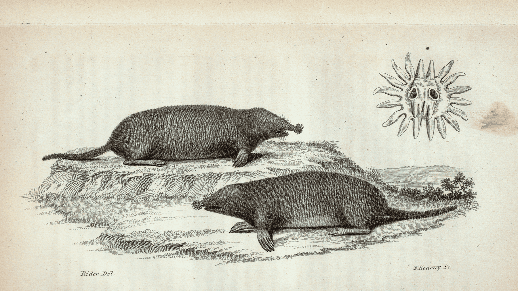
The star-nosed mole (Condylura cristata), found mainly in the northeastern United States and eastern Canada, has a unique and highly specialized nasal organ. Evolved over numerous generations, its nose consists of 22 tentacles with over 25,000 minute sensory receptors. Despite the moles being functionally blind, these tentacles allow them to create a detailed spatial map of their surroundings. They can navigate their dark underground habitat with astonishing precision and speed, quickly identifying and consuming edible items in a matter of milliseconds.

---

Congratulations! You’ve made it to the final act of this book. Take a moment to celebrate all that you’ve learned.

Throughout this book, you’ve explored the fundamental principles of interactive physics simulations with p5.js, dived into the complexities of agent and other rule-based behaviors, and dipped your toe into the exciting realm of machine learning. You’ve become a natural!

However, Chapter 10 merely scratched the surface of working with data and neural network–based machine learning—a vast landscape that would require countless sequels to this book to cover comprehensively. My goal was never to go deep into neural networks, but simply to establish the core concepts in preparation for a grand finale, where I find a way to integrate machine learning into the world of animated, interactive p5.js sketches and bring together as many of our new Nature of Code friends as possible for one last hurrah.

The path forward passes through the field of neuroevolution, a style of machine learning that combines the GAs from Chapter 9 with the neural networks from Chapter 10. A neuroevolutionary system uses Darwinian principles to evolve the weights (and in some cases, the structure itself) of a neural network over generations of trial-and-error learning. In this chapter, I’ll demonstrate how to use neuroevolution with a familiar example from the world of gaming. I’ll then finish off by varying Craig Reynolds’s steering behaviors from Chapter 5 so that they are learned through neuroevolution.

Reinforcement Learning

Neuroevolution shares many similarities with another machine learning methodology that I briefly referenced in Chapter 10, reinforcement learning, which incorporates machine learning into a simulated environment. A neural network–backed agent learns by interacting with the environment and receiving feedback about its decisions in the form of rewards or penalties. It’s a strategy built around observation.

Think of a little mouse running through a maze. If it turns left, it gets a piece of cheese; if it turns right, it receives a little shock. (Don’t worry, this is just a pretend mouse.) Presumably, the mouse will learn over time to turn left. Its biological neural network makes a decision with an outcome (turn left or right) and observes its environment (yum or ouch). If the observation is negative, the network can adjust its weights in order to make a different decision the next time.

In the real world, reinforcement learning is commonly used not for tormenting rodents but rather for developing robots. At time t, the robot performs a task and observes the results. Did it crash into a wall or fall off a table, or is it unharmed? As time goes on, the robot learns to interpret the signals from its environment in the optimal way to accomplish its tasks and avoid harm.

Instead of a mouse or a robot, now think about any of the example objects from earlier in this book (walker, mover, particle, vehicle). Imagine embedding a neural network into one of these objects and using it to calculate a force or another action. The neural network could receive its inputs from the environment (such as distance to an obstacle) and output some kind of decision. Perhaps the network chooses from a set of discrete options (move left or right) or picks a set of continuous values (the magnitude and direction of a steering force).

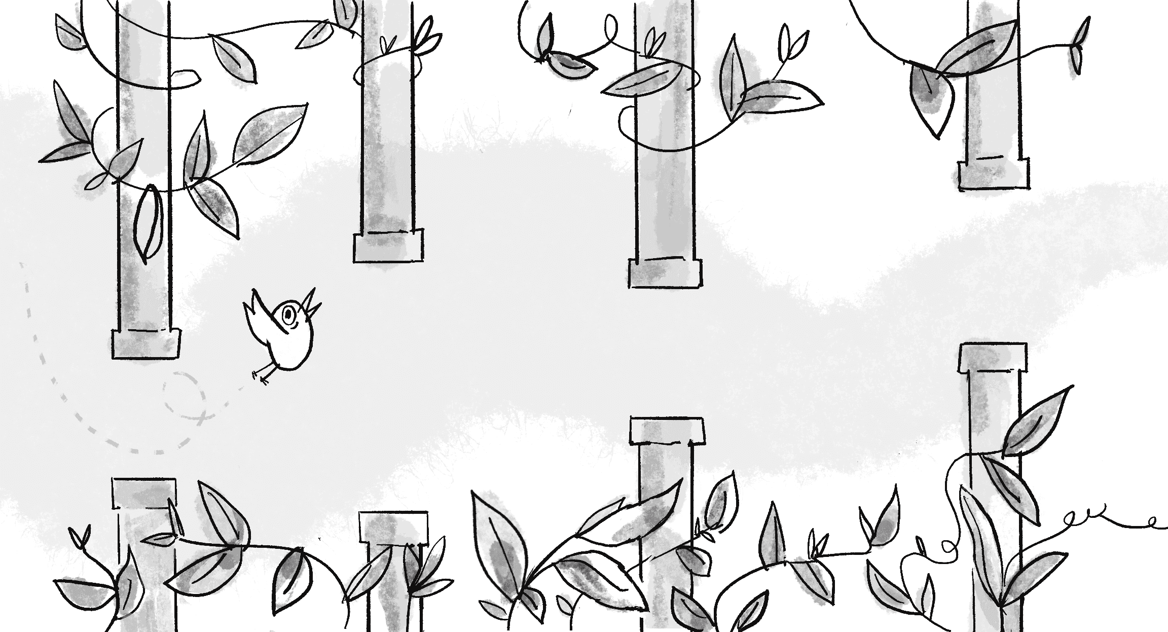
Is this starting to sound familiar? It’s no different from the way a neural network performed after training in the Chapter 10 examples, receiving inputs and predicting a classification or regression! Actually training one of these objects to make a good decision is where the reinforcement learning process diverges from the supervised learning approach. To better illustrate, let’s start with a hopefully easy-to-understand and possibly familiar scenario, the game Flappy Bird (see Figure 11.1).

The game is deceptively simple. You control a small bird that continually moves horizontally across the screen. With each tap or click, the bird flaps its wings and rises upward. The challenge? A series of vertical pipes spaced apart at irregular intervals emerge from the right. The pipes have gaps, and your primary objective is to navigate the bird safely through these gaps. If you hit a pipe, it’s game over. As you progress, the game’s speed increases, and the more pipes you navigate, the higher your score.

Suppose you want to automate the gameplay, and instead of a human tapping, a neural network will make the decision of whether to flap. Could machine learning work here? Skipping over the initial data steps in the machine learning life cycle for a moment, let’s think about how to choose a model. What are the inputs and outputs of the neural network?

This is quite the intriguing question because, at least in the case of the inputs, there isn’t a definitive answer. If you don’t know much about the game or don’t want to put your thumb on the scale in terms of identifying which aspects of the game are important, it might make the most sense to have the inputs be all the pixels of the game screen. This approach attempts to feed everything about the game into the model and let the model figure out for itself what matters.

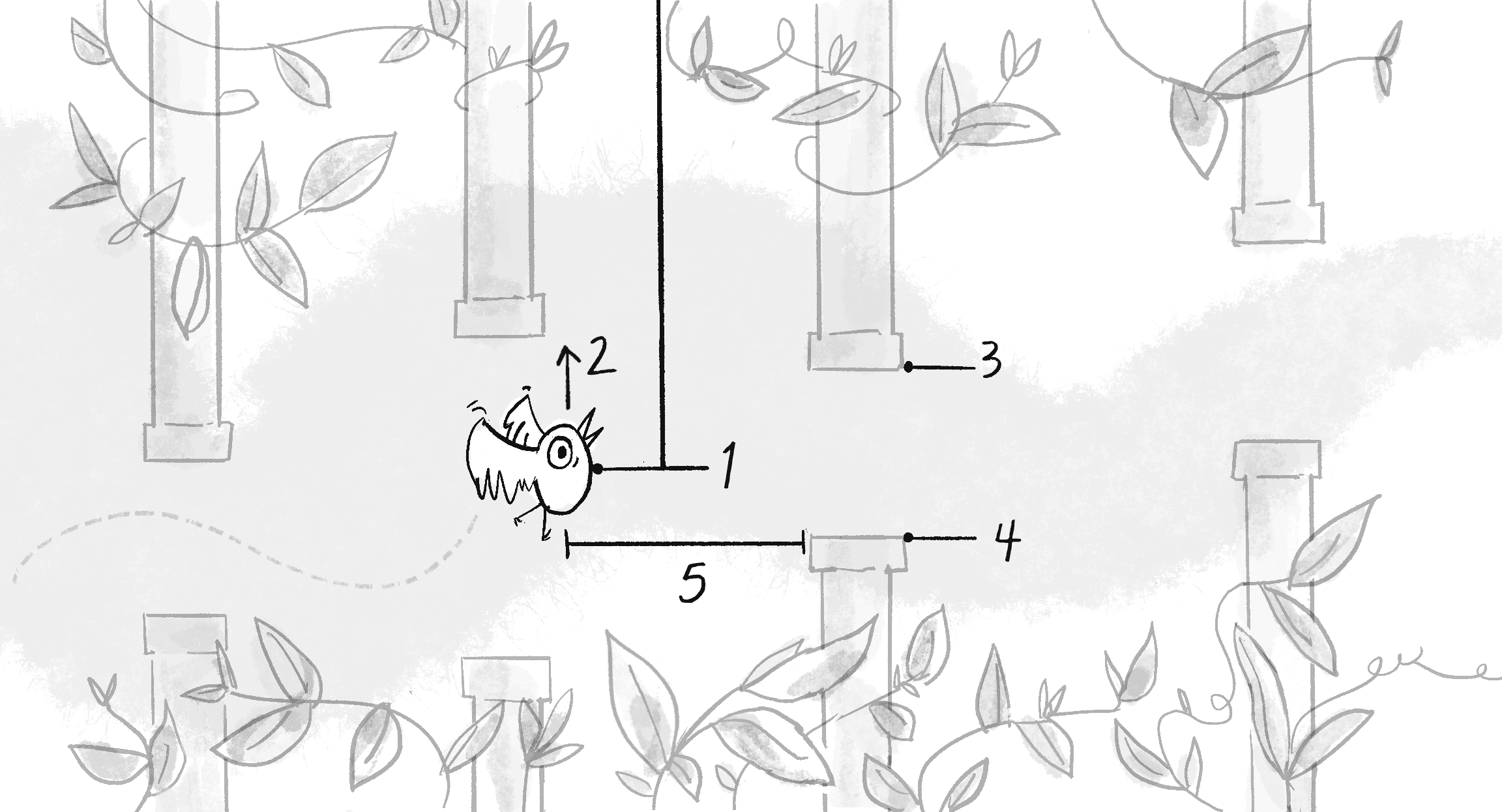
I’ve played Flappy Bird enough that I feel I understand it quite well, however. I can therefore bypass feeding all the pixels to the model and boil down the essence of the game to just a few input data points necessary for making predictions. These data points, often referred to as features in machine learning, represent the distinctive characteristics of the data that are most salient for the prediction. Imagine biting into a mysteriously juicy fruit—features like its taste (sweet!), texture (crisp!), and color (a vibrant red!) help you identify it as an apple. In the case of Flappy Bird, the most crucial features are listed here:

1. The y-position of the bird
2. The y-velocity of the bird
3. The y-position of the next top pipe’s opening

These features are illustrated in Figure 11.2.

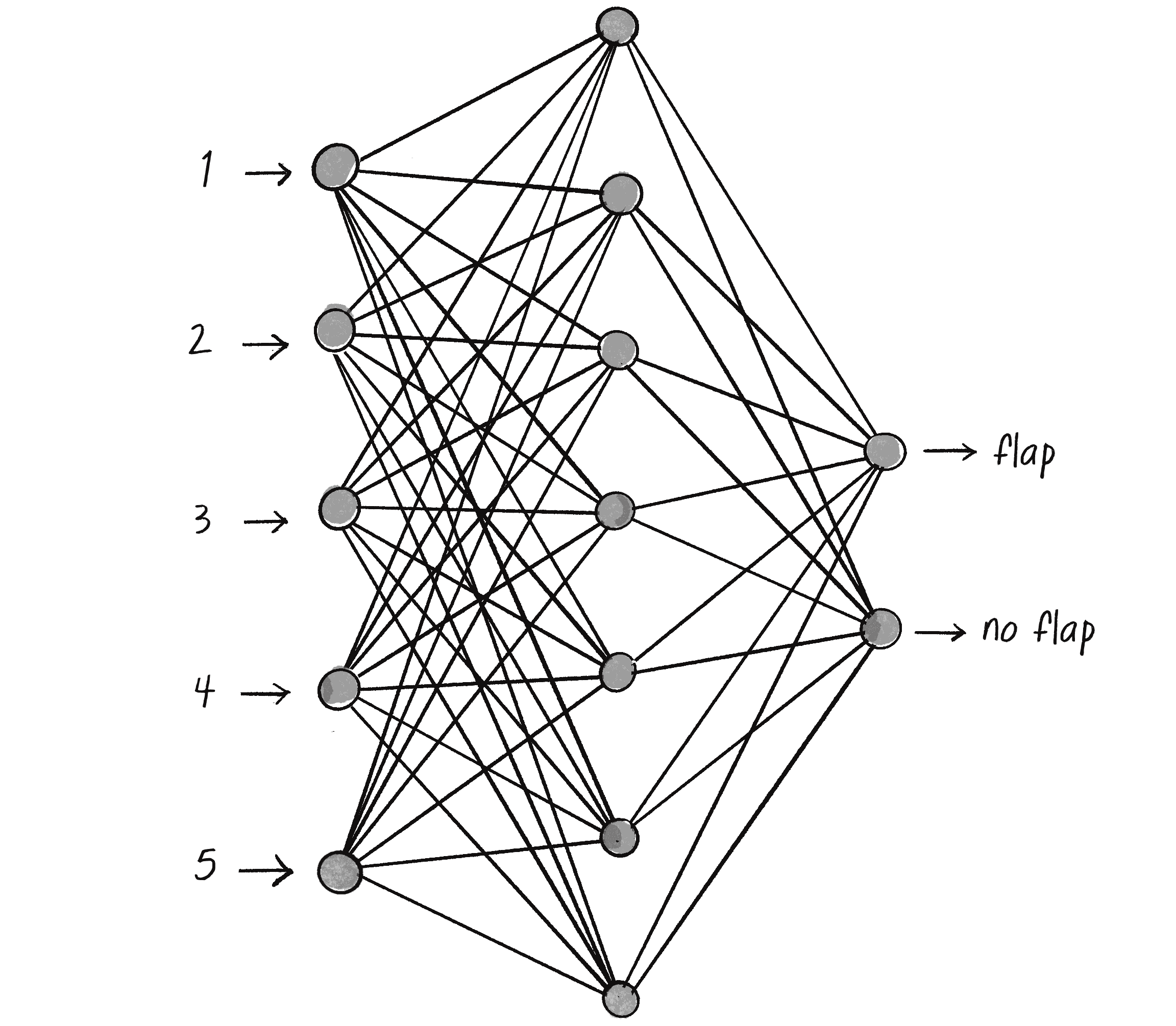
The neural network will have five inputs, one for each feature, but what about the outputs? Is this a classification problem or a regression problem? This may seem like an odd question to ask in the context of a game like Flappy Bird, but it’s actually quite important and relates to the way the game is controlled. Tapping the screen, pressing a button, or using keyboard controls are all examples of classification. After all, the player has only a discrete set of choices: tap or not; press W, A, S, or D on the keyboard. On the other hand, using an analog controller like a joystick leans toward regression. A joystick can be tilted in varying degrees in any direction, translating to continuous output values for both its horizontal and vertical axes.

For Flappy Bird, the outputs represent a classification decision with only two choices:

• Flap.
• Don’t flap.

This means the network should have two outputs, suggesting an overall network architecture like the one in Figure 11.3.

I now have all the information necessary to configure a model and let ml5.js build it:

let options = {

  inputs: 5,

  outputs: ["flap", "no flap"],

  task: "classification"

};

let birdBrain = ml5.neuralNetwork(options);

What next? If I were following the steps I laid out in Chapter 10, I’d have to go back to steps 1 and 2 of the machine learning process: data collection and preparation. How exactly would that work here? One idea could be to scour the earth for the greatest Flappy Bird player of all time and record them playing for hours. I could log the input features for every moment of gameplay along with whether the player flapped or not. Feed all that data into the model, train it, and I can see the headlines already: “Artificial Intelligence Bot Defeats Flappy Bird.”

But wait a second; has a computerized agent really learned to play Flappy Bird on its own, or has it simply learned to mirror the gameplay of a human? What if that human missed a key aspect of Flappy Bird strategy? The automated player would never discover it. Not to mention that collecting all that data would be incredibly tedious.

The problem here is that I’ve reverted to a supervised learning scenario like the ones from Chapter 10, but this is supposed to be a section about reinforcement learning. Unlike supervised learning, in which the correct answers are provided by a training dataset, the agent in reinforcement learning learns the answers—the optimal decisions—through trial and error by interacting with the environment and receiving feedback. In the case of Flappy Bird, the agent could receive a positive reward every time it successfully navigates a pipe, but a negative reward if it hits a pipe or the ground. The agent’s goal is to figure out which actions lead to the most cumulative rewards over time.

At the start, the Flappy Bird agent won’t know the best time to flap its wings, leading to many crashes. As it accrues more and more feedback from countless play-throughs, however, it will begin to refine its actions and develop the optimal strategy to navigate the pipes without crashing, maximizing its total reward. This process of learning by doing and optimizing based on feedback is the essence of reinforcement learning.

As the chapter goes on, I’ll explore the principles I’m outlining here, but with a twist. Traditional techniques in reinforcement learning involve defining a strategy (called a policy) and a corresponding reward function to provide feedback for adjusting the policy. Instead of going down this road, however, I’m going to turn toward the star of this chapter, neuroevolution.

Evolving Neural Networks Is NEAT!

Instead of using traditional backpropagation, a policy, and a reward function, neuroevolution applies principles of GAs and natural selection to train the weights in a neural network. This technique unleashes many neural networks on a problem at once. Periodically, the best-performing neural networks are “selected,” and their “genes” (the network connection weights) are combined and mutated to create the next generation of networks. Neuroevolution is especially effective in environments where the learning rules aren’t precisely defined or the task is complex, with numerous potential solutions.

One of the first examples of neuroevolution can be found in the 1994 paper “Genetic Lander: An Experiment in Accurate Neuro-genetic Control” by Edmund Ronald and Marc Schoenauer. In the 1990s, traditional neural network training methods were still nascent, and this work explored an alternative approach. The paper describes how a simulated spacecraft—in a game aptly named Lunar Lander—can learn how to safely descend and land on a surface. Rather than use handcrafted rules or labeled datasets, the researchers opted to use GAs to evolve and train neural networks over multiple generations. And it worked!

In 2002, Kenneth O. Stanley and Risto Miikkulainen expanded on earlier neuroevolutionary approaches with their paper “Evolving Neural Networks Through Augmenting Topologies”. Unlike the lunar lander method that focused on evolving the weights of a neural network, Stanley and Miikkulainen introduced a method that also evolved the network’s structure itself! Their NEAT algorithm—NeuroEvolution of Augmenting Topologies—starts with simple networks and progressively refines their topology through evolution. As a result, NEAT can discover network architectures tailored to specific tasks, often yielding more optimized and effective solutions.

A comprehensive NEAT implementation would require going deeper into neural network architectures and working directly with TensorFlow.js. My goal instead is to emulate Ronald and Schoenauer’s original research in the modern context of the web browser with ml5.js. Rather than use the Lunar Lander game, I’ll give this a try with Flappy Bird. And for that, I first need to code a version of Flappy Bird where my neuroevolutionary network can operate.

Coding Flappy Bird

Flappy Bird was created by Vietnamese game developer Dong Nguyen in 2013. In January 2014, it became the most downloaded app on the Apple App Store. However, on February 8 of that year, Nguyen announced that he was removing the game because of its addictive nature. Since then, it has become one of the most cloned games in history.

Flappy Bird is a perfect example of Nolan’s law, an aphorism attributed to the founder of Atari and creator of Pong, Nolan Bushnell: “All the best games are easy to learn and difficult to master.” It’s also a terrific game for beginner coders to re-create as a learning exercise, and it fits perfectly with the concepts in this book.

To program the game with p5.js, I’ll start by defining a Bird class. This may shock you, but I’m going to skip using p5.Vector for this demonstration and instead use separate x and y properties for the bird’s position. Since the bird moves only along the vertical axis in the game, x remains constant! Therefore, the velocity (and all the relevant forces) can be a single scalar value for just the y-axis.

To simplify the code even further, I’ll add the forces directly to the bird’s velocity instead of accumulating them into an acceleration variable. In addition to the usual update(), I’ll include a flap() method for the bird to fly upward. The show() method isn’t included here as it only draws a circle. Here’s the code:

class Bird {

  constructor() {

    this.x = 50
    this.y = 120;

    this.velocity = 0;
    this.gravity = 0.5;
    this.flapForce = -10;

  }

  flap() {
    this.velocity += this.flapForce;
  }

  update() {

    this.velocity += this.gravity;
    this.y += this.velocity;

    this.velocity *= 0.95;

    if (this.y > height) {
      this.y = height;
      this.velocity = 0;
    }

  }

}

The other primary elements of the game are the pipes that the bird must navigate through. I’ll create a Pipe class to describe a pair of rectangles, one that emanates from the top of the canvas and one from the bottom. Just as the bird moves only vertically, the pipes slide along only the horizontal axis, so the properties can also be scalar values rather than vectors. The pipes move at a constant speed and don’t experience any other forces.

class Pipe {

  constructor() {

    this.spacing = 100;

    this.top = random(height - this.spacing);

    this.bottom = this.top + this.spacing;

    this.x = width;

    this.w = 20;

    this.velocity = 2;

  }

  show() {
    fill(0);
    noStroke();
    rect(this.x, 0, this.w, this.top);
    rect(this.x, this.bottom, this.w, height - this.bottom);
  }

  update() {
    this.x -= this.velocity;
  }

}

To be clear, the game depicts a bird flying through pipes—the bird is moving along two dimensions while the pipes remain stationary. However, it’s simpler to code the game as if the bird is stationary in its horizontal position and the pipes are moving.

With a Bird and Pipe class written, I’m almost set to run the game. However, a key piece is missing: collisions. The whole game rides on the bird attempting to avoid the pipes! Fortunately, this is nothing new. You’ve seen many examples of objects checking their positions against others throughout this book. I have a design choice to make, though. A method to check collisions could logically be placed in either the Bird class (to check whether the bird hits a pipe) or the Pipe class (to check whether a pipe hits the bird). Either can be justified, depending on your point of view.

I’ll place the method in the Pipe class and call it collides(). The code itself is a little trickier than you might think at first glance, as the method needs to check both the top and bottom rectangles of a pipe against the position of the bird. I could approach this in a variety of ways. One way is to first check whether the bird is vertically within the bounds of either rectangle (either above the bottom of the top pipe or below the top of the bottom one). But the bird is colliding with the pipe only if the bird is also horizontally within the boundaries of the pipe’s width. An elegant way to write this is to combine each of these checks with a logical and:

  collides(bird) {

    let verticalCollision = bird.y < this.top || bird.y > this.bottom;

    let horizontalCollision = bird.x > this.x && bird.x < this.x + this.w;

    return verticalCollision && horizontalCollision;

  }

The algorithm currently treats the bird as a single point and doesn’t take into account its size. This detail should be improved for a more realistic version of the game.

All that’s left is to write setup() and draw(). I need a single variable for the bird and an array for a list of pipes. The interaction is just a single click of the mouse, which triggers the bird’s flap() method. Rather than build a fully functional game with a score, end screen, and other usual elements, I’ll just make sure that the game mechanics are working by drawing the text OOPS! near any pipe when a collision occurs. The code also assumes an additional offscreen() method on the Pipe class for when a pipe has moved beyond the left edge of the canvas.

let bird;

let pipes = [];

function setup() {

  createCanvas(640, 240);

  bird = new Bird();
  pipes.push(new Pipe());

}

function mousePressed() {
  bird.flap();
}

function draw() {

  background(255);

  for (let i = pipes.length - 1; i >= 0; i--) {
    pipes[i].show();
    pipes[i].update();
    if (pipes[i].collides(bird)) {
      text("OOPS!", pipes[i].x, pipes[i].top + 20);
    }
    if (pipes[i].offscreen()) {
      pipes.splice(i, 1);
    }
  }

  bird.update();
  bird.show();

  if (frameCount % 100 === 0) {
    pipes.push(new Pipe());
  }

}

The trickiest aspect of this code lies in spawning the pipes at regular intervals with the frameCount variable and modulo operator. In p5.js, frameCount is a system variable that tracks the number of frames rendered since the sketch began, incrementing with each cycle of the draw() loop. The modulo operator, denoted by %, returns the remainder of a division operation. For example, 7 % 3 yields 1 because when dividing 7 by 3, the result is 2 with a remainder of 1. The Boolean expression frameCount % 100 === 0 therefore checks whether the current frameCount value, when divided by 100, has a remainder of 0. This condition is true every 100 frames, and at those frames, a new pipe is spawned and added to the pipes array.

Neuroevolutionary Flappy Bird

My Flappy Bird clone, as it currently stands, is controlled by mouse clicks. Now I want to cede control of the game to the computer and use neuroevolution to teach it how to play. Luckily, the process of neuroevolution is already baked into ml5.js, so making this switch will be relatively straightforward. The first step is to give the bird a brain so it can decide on its own whether to flap its wings.

The Bird Brain

When I introduced reinforcement learning, I established a list of input features that should make up the bird’s decision-making process. I’m going to use that same list but with one simplification. Since the size of the opening between the pipes is constant, there’s no need to include the y-positions of both the top and bottom; one or the other will suffice. The input features are therefore as follows:

1. The y-position of the bird
2. The y-velocity of the bird
3. The y-position of the next pipe’s top (or bottom!) opening
4. The x-distance to the next pipe

The two outputs represent the bird’s two options: to flap or not to flap. With the inputs and outputs set, I can add a brain property to the bird’s constructor to hold an ml5.js neural network with the appropriate configuration. Just to demonstrate a different coding style here, I’ll skip including a separate options variable and pass the properties as an object literal directly into the ml5.neuralNetwork() function. Note the addition of a neuroEvolution property set to true. This is necessary to enable some of the features I’ll be using later in the code.

  constructor() {

    this.brain = ml5.neuralNetwork({

      inputs: 4,
      outputs: ["flap", "no flap"],
      task: "classification",

      neuroEvolution: true

    });

  }

Next, I’ll add a new method called think() to the Bird class to calculate all the necessary inputs for the bird at each moment in time. The first two inputs are easy—they’re simply the y and velocity properties of the bird. However, for inputs 3 and 4, I need to determine which pipe is the next pipe.

At first glance, it might seem that the next pipe is always the first one in the array, since the pipes are added one at a time to the end of the array. However, after a pipe passes the bird, it’s no longer relevant, and there’s still some time between when this happens and when that pipe exits the canvas and is removed from the beginning of the array. I therefore need to find the first pipe in the array whose right edge (x-position plus width) is greater than the bird’s x-position:

  think(pipes) {

    let nextPipe = null;

    for (let pipe of pipes) {

      if (pipe.x + pipe.w > this.x) {
        nextPipe = pipe;
        break;
      }

    }

Once I have the next pipe, I can create the four inputs:

    let inputs = [

      this.y,

      this.velocity,

      nextPipe.top,

      nextPipe.x - this.x,

    ];

This is close, but I’ve forgotten a critical step. The range of all input values is determined by the dimensions of the canvas, but a neural network expects values in a standardized range, such as 0 to 1. One method to normalize these values is to divide the inputs related to vertical properties by height, and those related to horizontal ones by width:

    let inputs = [

      this.y / height,
      this.velocity / height,
      nextPipe.top / height,
      (nextPipe.x - this.x) / width,

    ];

With the inputs in hand, I’m ready to pass them to the neural network’s classify() method. I have another small problem, however: classify() is asynchronous, meaning I’d have to implement a callback inside the Bird class to process the model’s decision. This would add a significant level of complexity to the code, but luckily, it’s entirely unnecessary in this case. Asynchronous callbacks with ml5.js’s machine learning functions are typically needed because of the time required to process the large amount of data in the model. Without a callback, the code might have to wait a long time to get a result, and if the model is running as part of a p5.js sketch, that delay could severely impact the smoothness of the animation. The neural network here, however, has only four floating-point
inputs and two output labels! It’s tiny and can run fast enough that there’s no reason to use asynchronous code.

    let results = this.brain.classifySync(inputs);

    if (results[0].label === "flap") {

      this.flap();

    }

  }

The neural network’s prediction is in the same format as the gesture classifier from Chapter 10, and the decision can be made by checking the first element of the results array. If the output label is "flap", then call flap().

Now that I’ve finished the think() method, the real challenge can begin: teaching the bird to win the game by consistently flapping its wings at the right moment. This is where the GA comes back into the picture. Recalling the discussion from Chapter 9, three key principles underpin Darwinian evolution: variation, selection, and heredity. I’ll revisit each of these principles in turn as I implement the steps of the GA in this new context of neural networks.

Variation: A Flock of Flappy Birds

A single bird with a randomly initialized neural network isn’t likely to have any success at all. That lone bird will most likely jump incessantly and fly way off-screen, or sit perched at the bottom of the canvas awaiting collision after collision with the pipes. This erratic and nonsensical behavior is a reminder: a randomly initialized neural network lacks any knowledge or experience. The bird is essentially making wild guesses for its actions, so success is going to be rare.

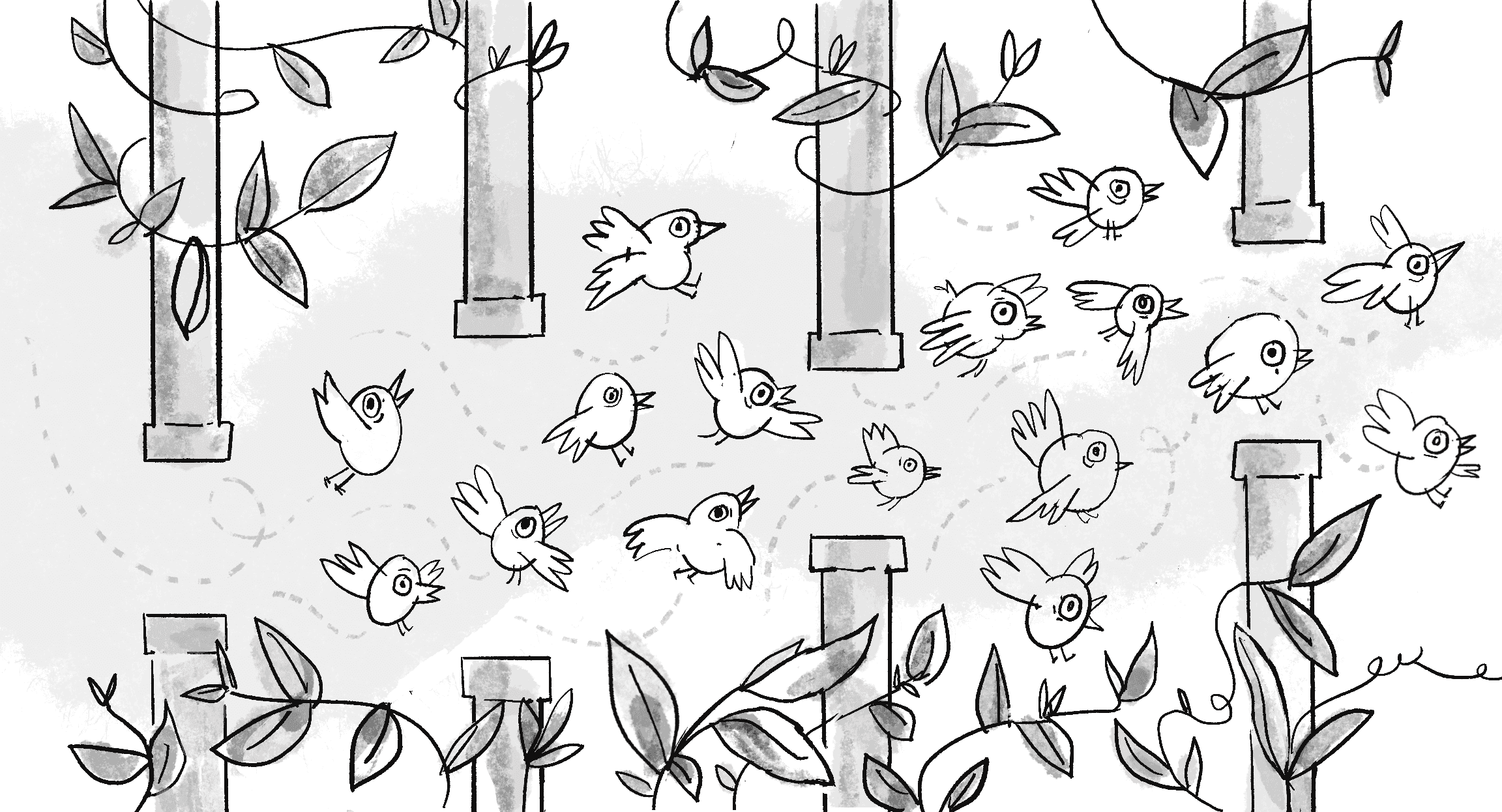
This is where the first key principle of GAs comes in: variation. The hope is that by introducing as many different neural network configurations as possible, a few might perform slightly better than the rest. The first step toward variation is to add an array of many birds (Figure 11.4).

let populationSize = 200;

let birds = [];

function setup() {

  for (let i = 0; i < populationSize; i++) {
    birds[i] = new Bird();
  }

  ml5.setBackend("cpu");

}

function draw() {

  for (let bird of birds) {

    bird.think(pipes);

    bird.update();

    bird.show();

  }

}

You might notice a peculiar line of code that’s crept into the setup() function: ml5.setBackend("cpu"). When running neural networks, a lot of the heavy computational lifting is often offloaded to the GPU. This is the default behavior, and it’s especially critical for the larger pretrained models included with ml5.js.

But there’s a catch! Transferring data to and from the GPU introduces overhead. In most cases,
the gains from the GPU’s parallel processing more than offset this overhead, but for a tiny model
like the one here, copying data to the GPU and back actually slows the neural network. Calling ml5.setBackend("cpu") tells ml5.js to run the neural network computations on the CPU instead. At least in this simple case of tiny bird brains, this is the more efficient choice.

Selection: Flappy Bird Fitness

Once I have a diverse population of birds, each with its own neural network, the next step in the GA is selection. Which birds should pass on their genes (in this case, neural network weights) to the next generation? In the world of Flappy Bird, the measure of success is the ability to stay alive the longest by avoiding the pipes. This is the bird’s fitness. A bird that dodges many pipes is considered more fit than one that crashes into the first pipe it encounters.

To track each bird’s fitness, I’ll add two properties to the Bird class, fitness and alive:

  constructor() {

    this.fitness = 0;

    this.alive = true;

  }

I’ll assign the fitness a numeric value that increases by one every cycle through draw(), as long as the bird remains alive. The birds that survive longer should have a higher fitness value. This mechanism mirrors the reinforcement learning technique of rewarding good decisions. In reinforcement learning, however, an agent receives immediate feedback for every decision it makes, allowing it to adjust its policy accordingly. Here, the bird’s fitness is a cumulative measure of its overall success and will be applied only during the selection step of the GA.

  update() {

    this.fitness++;

  }

The alive property is a Boolean flag that’s initially set to true. When a bird collides with a pipe, this property is set to false. Only birds that are still alive are updated and drawn to the canvas.

function draw() {

  for (let bird of birds) {

    if (bird.alive) {

      bird.think(pipes);

      bird.update();
      bird.show();

      for (let pipe of pipes) {  
        if (pipe.collides(bird)) {
          bird.alive = false;
        }

      }

    }

  }

}

In Chapter 9, I demonstrated two techniques for running an evolutionary simulation. In the smart rockets example, the population lived for a fixed amount of time each generation. The same approach could likely work here as well, but I want to allow the birds to accumulate the highest fitness value possible and not arbitrarily stop them based on a time limit. The second technique, demonstrated with the bloops example, eliminated the fitness score entirely and set a random probability for cloning any living creature. For Flappy Bird, this approach could become messy and risks overpopulation or all the birds dying out completely.

I propose combining elements of both approaches. I’ll allow a generation to continue as long as at least one bird is still alive. When all the birds have died, I’ll select parents for the reproduction step and start anew. I’ll begin by writing a function to check whether all the birds have died:

function allBirdsDead() {

  for (let bird of birds) {

    if (bird.alive) {
      return false;
    }

  }

  return true;

}

When all the birds have died, it’s time for selection! In the previous GA examples, I demonstrated a relay-race technique for giving a fair shot to all members of a population, while still increasing the chances of selection for those with higher fitness scores. I’ll use that same weightedSelection() function here:

function weightedSelection() {

  let index = 0;

  let start = random(1);

  while (start > 0) {

    start = start - birds[index].fitness;

    index++;

  }

  index--;

  return birds[index].brain;

}

For this algorithm to function properly, I need to first normalize the fitness values of the birds so that they collectively add up to 1:

function normalizeFitness() {

  let sum = 0;
  for (let bird of birds) {
    sum += bird.fitness;
  }

  for (let bird of birds) {
    bird.fitness = bird.fitness / sum;
  }

}

Once normalized, each bird’s fitness is equal to its probability of being selected.

Heredity: Baby Birds

Only one step is left in the GA—reproduction. In Chapter 9, I explored in great detail the two-step process for generating a child element: crossover and mutation. Crossover is where the third key principle of heredity arrives: the DNA from the two selected parents is combined to form the
child’s DNA.

At first glance, the idea of inventing a crossover algorithm for two neural networks might seem daunting, and yet it’s quite straightforward. Think of the individual “genes” of a bird’s brain as the weights within the neural network. Mixing two such brains boils down to creating a new neural network with each weight chosen by a virtual coin flip—the weight comes from either the first or the second parent:

let parentA = weightedSelection();
let parentB = weightedSelection();
let child = parentA.crossover(parentB);

Wow, today’s my lucky day! It turns out ml5.js includes a crossover() method that manages the algorithm for mixing the two neural networks. I can happily move on to the mutation step:

child.mutate(0.01);

My luck continues! The ml5.js library also provides a mutate() method that accepts a mutation rate as its primary argument. The rate determines how often a weight will be altered. For example, a rate of 0.01 indicates a 1 percent chance that any given weight will mutate. During mutation, ml5.js adjusts the weight slightly by adding a small random number to it, rather than selecting a completely new random value. This behavior mimics real-world genetic mutations, which typically introduce minor changes rather than entirely new traits. Although this default approach works for many cases, ml5.js offers more control over the process by allowing the use of a custom mutation function as an optional second argument to mutate().

The crossover and mutation steps need to be repeated for the size of the population to create an entirely new generation of birds. This is accomplished by populating an empty local array nextBirds with the new birds. Once the population is full, the global birds array is then updated to this fresh generation:

function reproduction() {

  let nextBirds = [];

  for (let i = 0; i < populationSize; i++) {

    let parentA = weightedSelection();
    let parentB = weightedSelection();

    let child = parentA.crossover(parentB);

    child.mutate(0.01);

    nextBirds[i] = new Bird(child);

  }

  birds = nextBirds;

}

If you look closely at the reproduction() function, you may notice that I’ve slipped in another new feature of the Bird class: an argument to the constructor. When I first introduced the idea of a bird brain, each new Bird object was created with a brand-new brain—a fresh neural network courtesy of ml5.js. However, I now want the new birds to inherit a child brain that was generated through the processes of crossover and mutation. To make this possible, I’ll subtly change the Bird constructor to look for an optional argument named, of course, brain:

  constructor(brain) {

    if (brain) {

      this.brain = brain;

    } else {

      this.brain = ml5.neuralNetwork({

        inputs: 4,

        outputs: ["flap", "no flap"],

        task: "classification",

        neuroEvolution: true,

      });

    }

  }

If no brain is provided when a new bird is created, the brain argument remains undefined. In JavaScript, undefined is treated as false. The if (brain) test will therefore fail, so the code will move on to the else statement and call ml5.neuralNetwork(). On the other hand, if an existing neural network is passed in, brain evaluates to true and is assigned directly to this.brain. This elegant trick allows a single constructor to handle multiple scenarios.

With that, the example is complete. All that’s left to do is call normalizeFitness() and reproduction() in draw() at the end of each generation, when all the birds have died out.

function draw() {

  /* All the rest of draw */

  if (allBirdsDead()) {
    normalizeFitness();
    reproduction();
    resetPipes();

  }

}

function resetPipes() {

  pipes.splice(0, pipes.length - 1);

}

Note the addition of a new resetPipes() function. If I don’t remove the pipes before starting a new generation, the birds may immediately restart at a position colliding with a pipe, in which case even the best bird won’t have a chance to fly! The full online code for Example 11.2 also adjusts the behavior of the birds so that they die when they leave the canvas, either by crashing into the ground or soaring too high above the top.

Steering the Neuroevolutionary Way

Having explored neuroevolution with Flappy Bird, I’d like to shift the focus back to the realm of simulation, specifically the steering agents introduced in Chapter 5. What if, instead of me dictating the rules for an algorithm to calculate a steering force, a simulated creature could evolve its own strategy? Drawing inspiration from Reynolds’s aim of lifelike and improvisational behaviors, my goal isn’t to use neuroevolution to engineer the perfect creature that can flawlessly execute a task. Instead, I hope to create a captivating world of simulated life, where the quirks, nuances, and happy accidents of evolution unfold in the canvas.

I’ll begin by adapting the smart rockets example from Chapter 9. In that example, the genes for each rocket were an array of vectors:

this.genes = [];

for (let i = 0; i < lifeSpan; i++) {

  this.genes[i] = p5.Vector.random2D();
  this.genes[i].mult(random(0, this.maxforce));

}

I propose adapting this code to instead use a neural network to predict the vector or steering force, transforming the genes into a brain. Vectors can have a continuous range of values, so this is a regression task:

this.brain = ml5.neuralNetwork({

  inputs: 2,

  outputs: 2,

  task: "regression",

  neuroEvolution: true,

});

In the original example, the vectors from the genes array were applied sequentially, querying the array with a counter variable:

this.applyForce(this.genes[this.counter]);

Now, instead of an array lookup, I want the neural network to return a new vector for each frame of the animation. For regression tasks with ml5.js, the output of the neural network is received from the predict() method rather than classify(). And here, I’ll use the predictSync() variant to keep the code simple and allow for synchronous output data from the model in the rocket’s run() method:

run() {

  let outputs = this.brain.predictSync(inputs);

  let angle = outputs[0].value * TWO_PI;

  let magnitude = outputs[1].value * this.maxforce;

  let force = p5.Vector.fromAngle(angle)
  force.setMag(magnitude);
  this.applyForce(force);

}

The neural network brain outputs two values: one for the angle of the vector and one for the magnitude. You might think to instead use these outputs for the vector’s x- and y-components. The default output range for an ml5.js neural network is from 0 to 1, however, and I want the forces to be capable of pointing in both positive and negative directions. Mapping the first output to an angle by multiplying it by TWO_PI offers the full range.

You may have noticed that the code includes a variable called inputs that I have yet to declare or initialize. Defining the inputs to the neural network is where you, as the designer of the system, can be the most creative. You have to consider the nature of the environment and the simulated biology and capabilities of your creatures, and then decide which features are most important.

As a first try, I’ll assign something basic for the inputs and see if it works. Since the smart rockets’ environment is static, with fixed obstacles and targets, what if the brain could learn and estimate a flow field to navigate toward its goal? As I demonstrated in Chapter 5, a flow field receives a position and returns a vector, so the neural network can mirror this functionality and use the rocket’s current x- and y-position as input. I just have to normalize the values according to the canvas dimensions:

let inputs = [this.position.x / width, this.position.y / height];

That’s it! Virtually everything else from the original example can remain unchanged: the population, the fitness function, and the selection process.

  reproduction() {

    let nextPopulation = [];

    for (let i = 0; i < this.population.length; i++) {

      let parentA = this.weightedSelection();
      let parentB = this.weightedSelection();
      let child = parentA.crossover(parentB);

      child.mutate(this.mutationRate);

      nextPopulation[i] = new Rocket(320, 220, child);

    }

    this.population = nextPopulation;

    this.generations++;

  }

Now that I’m using ml5.js, notice that I no longer need a separate DNA class with implementations of crossover() and mutate(). Instead, those methods are built into ml5.neuralNetwork and can be called directly.

Responding to Change

In the previous example, the environment was static, with a stationary target and obstacle. This made the rocket’s task of finding the target easy to accomplish using only its position as input. However, what if the target and the obstacles in the rocket’s path were moving? To handle a more complex and changing environment, I need to expand the neural network’s inputs and consider additional features of the environment. This is similar to what I did with Flappy Bird, as I identified the key data points of the environment to guide the bird’s decision-making process.

I’ll begin with the simplest version of this scenario, almost identical to the original smart rockets example, but removing obstacles and replacing the fixed target with a random walker controlled by Perlin noise. In this world, I’ll rename the Rocket to Creature and recast the walker as a Glow class that represents a gentle, drifting orb. Imagine that the creature’s goal is to reach the light source and dance in its radiant embrace as long as it can:

class Glow {

  constructor() {

    this.xoff = 0;
    this.yoff = 1000;

    this.position = createVector();

    this.r = 24;

  }

  update() {

    this.position.x = noise(this.xoff) * width;
    this.position.y = noise(this.yoff) * height;

    this.xoff += 0.01;
    this.yoff += 0.01;

  }

  show() {

    stroke(0);

    strokeWeight(2);

    fill(200);

    circle(this.position.x, this.position.y, this.r * 2);

  }

}

As the glow moves, the creature should take the glow’s position into account in its decision-making process, as an input to its brain. However, it isn’t sufficient to know only the light’s position; it’s the position relative to the creature’s own that’s key. A nice way to synthesize this information as an input feature is to calculate a vector that points from the creature to the glow. Essentially, I’m reinventing the seek() method from Chapter 5, using a neural network to estimate the steering force:

  seek(target) {

    let v = p5.Vector.sub(target.position, this.position);

This is a good start, but the components of the vector don’t fall within a normalized input range. I could divide v.x by width and v.y by height, but since my canvas isn’t a perfect square, this may skew the data. Another solution is to normalize the vector, but while this would retain information about the direction from the creature to the glow, it would eliminate any measure of the distance. This won’t do either—if the creature is sitting on top of the glow, it should steer differently than if it were very far away. As a solution, I’ll save the distance in a separate variable before normalizing the vector. For it to work as an input feature, though, I still have to normalize the range. While not a perfect normalization from 0 to 1, I’ll divide it by the canvas width, which will provide a practical normalization that retains the relative magnitude:

  seek(target) {

    let v = p5.Vector.sub(target.position, this.position);

    let distance = v.mag() / width;

    v.normalize();

As you may recall, a key element of Reynolds’s steering formula involved comparing the desired velocity to the current velocity. How the vehicle is currently moving plays a significant role in how it should steer! For the creature to consider its own velocity as part of its decision-making, I can include the velocity vector in the inputs to the neural network as well. To normalize these values, dividing the vector’s components by the maxspeed property works beautifully. This retains both the direction and relative magnitude of the vector. The rest of the seek() method follows the same logic as the previous example, with the outputs of the neural network synthesized into a force to be applied to the creature:

  seek(target) {

    let v = p5.Vector.sub(target.position, this.position);

    let distance = v.mag() / width;

    v.normalize();

    let inputs = [
      v.x,
      v.y,
      distance,
      this.velocity.x / this.maxspeed,
      this.velocity.y / this.maxspeed,
    ];

    let outputs = this.brain.predictSync(inputs);
    let angle = outputs[0].value * TWO_PI;
    let force = p5.Vector.fromAngle(angle);
    let magnitude = outputs[1].value;
    force.setMag(magnitude);

    this.applyForce(force);

  }

Enough has changed in the transition from rockets to creatures that it’s also worth reconsidering the fitness function. Previously, fitness was calculated based on the rocket’s record distance from the target at the end of each generation. Since the target is now moving, I’d prefer to accumulate the amount of time the creature is able to catch the glow as the measure of fitness. This can be achieved by checking the distance between the creature and the glow in the update() method and incrementing a fitness value when they’re intersecting:

  update(target) {

    /* The usual updating of position, velocity, acceleration */

    let d = p5.Vector.dist(this.position, target.position);
    if (d < this.r + target.r) {
      this.fitness++;
    }

  }

Both the Glow and Creature classes include a radius property r, which I’m using to determine intersection.

Speeding Up Time

One thing you may have noticed about evolutionary computing is that testing the code is a delightful exercise in patience. You have to watch the slow crawl of the simulation play out generation after generation. This is part of the point—I want to watch the process! It’s also a nice excuse to take a break, which is to be encouraged. Head outside and enjoy some nonsimulated nature for a while, or perhaps a soothing cup of tea. Then check back in on your creatures and see how they’re progressing. Take comfort in having to wait only billions of milliseconds rather than the billions of years required for actual biological evolution.

Nevertheless, for the system to evolve, there’s no inherent requirement that you draw and animate the world. Hundreds of generations could be completed in the blink of an eye if you could skip all the time spent rendering the scene. Or, rather than not render the environment at all, you could choose to simply render it less often. This will save you from tearing your hair out every time you change a small parameter and find yourself waiting what seems like hours to see whether it had any effect on the system’s evolution.

Here’s where I can use one of my favorite features of p5.js: the ability to quickly create standard interface elements. You saw this before in Example 9.4 with createButton(). This time I’ll create a slider to control the number of iterations of a for loop that runs inside draw(). The for loop will contain the code for updating (but not drawing) the simulation. The more times the loop repeats, the faster the animation will seem.

Here’s the code for this new time slider, excluding all the other global variables and their initializations in setup(). Notice that the code for the visuals is separated from the code for the physics to ensure that rendering still occurs only once per draw() cycle:

let timeSlider;

function setup() {

  timeSlider = createSlider(1, 20, 1);

}

function draw() {

  background(255);
  glow.show();
  for (let creature of creatures) {
    creature.show();
  }

  for (let i = 0; i < timeSlider.value(); i++) {
    for (let creature of creatures) {
      creature.seek(glow);
      creature.update(glow);
    }
    glow.update();
    lifeCounter++;
  }

}

In p5.js, a slider is defined with three arguments: a minimum value (for when the slider is all the way to the left), a maximum value (for when it’s all the way to the right), and a starting value (for when the page first loads). In this case, the slider allows you to run the simulation at 20x speed to reach the results of evolution more quickly, then slow it back down to 1x speed to bask in the glory of the intelligent behaviors on display.

Here’s the final version of the example with a new Creature constructor to create a neural network. Everything else related to applying the steps of the GA has remained the same from the Flappy Bird example code.

class Creature {

  constructor(x, y, brain) {

    this.position = createVector(x, y);

    this.velocity = createVector(0, 0);

    this.acceleration = createVector(0, 0);

    this.r = 4;

    this.maxspeed = 4;

    this.fitness = 0;

    if (brain) {

      this.brain = brain;

    } else {

      this.brain = ml5.neuralNetwork({

        inputs: 5,

        outputs: 2,

        task: "regression",

        neuroEvolution: true,

      });

    }

  }

  /* seek() predicts a steering force as described previously. */

  /* update() increments the fitness if the glow is reached as described previously. */

}

It’s hard to believe, but this book has been a journey well over 10 years in the making. Thank you, dear reader, for sticking with it. I promise it’s not an infinite loop. However meandering it might have seemed, like a random walk, I’m finally using an arrival steering behavior to reach the final piece of the puzzle, an attempt to bring together all my past explorations in my own version of the Ecosystem Project.

A Neuroevolutionary Ecosystem

A few elements in this chapter’s examples don’t quite fit with my dream of simulating a natural ecosystem. The first goes back to an issue I raised in Chapter 9 with the introduction of the bloops. A system of creatures that all live and die together, starting completely over with each subsequent generation—that isn’t how the biological world works! I’d like to revisit this dilemma in this chapter’s context of neuroevolution.

Second, and perhaps more important, a major flaw exists in the way I’m extracting features from a scene to train a model. The creatures in Example 11.4 are all-knowing. Sure, it’s reasonable to assume that a creature is aware of its own current velocity, but I’ve also allowed each creature to know the glow’s exact location, regardless of how far away it is or what might be blocking the creature’s vision or senses. This is a bridge too far. It flies in the face of one of the main tenets of autonomous agents I introduced in Chapter 5: an agent should have a limited ability to perceive its environment.

Sensing the Environment

A common approach to simulating how a real-world creature (or robot) would have a limited awareness of its surroundings is to attach sensors to an agent. Think back to that mouse in the maze from the beginning of the chapter (hopefully it’s been thriving on the cheese it’s been getting as a reward), and now imagine it has to navigate the maze in the dark. Its whiskers might act as proximity sensors to detect walls and turns. The mouse whiskers can’t see the entire maze, but only sense the immediate surroundings. Another example of sensors is a bat using echolocation to navigate, or a car on a winding road where the driver can see only what’s projected in front of the car’s headlights.

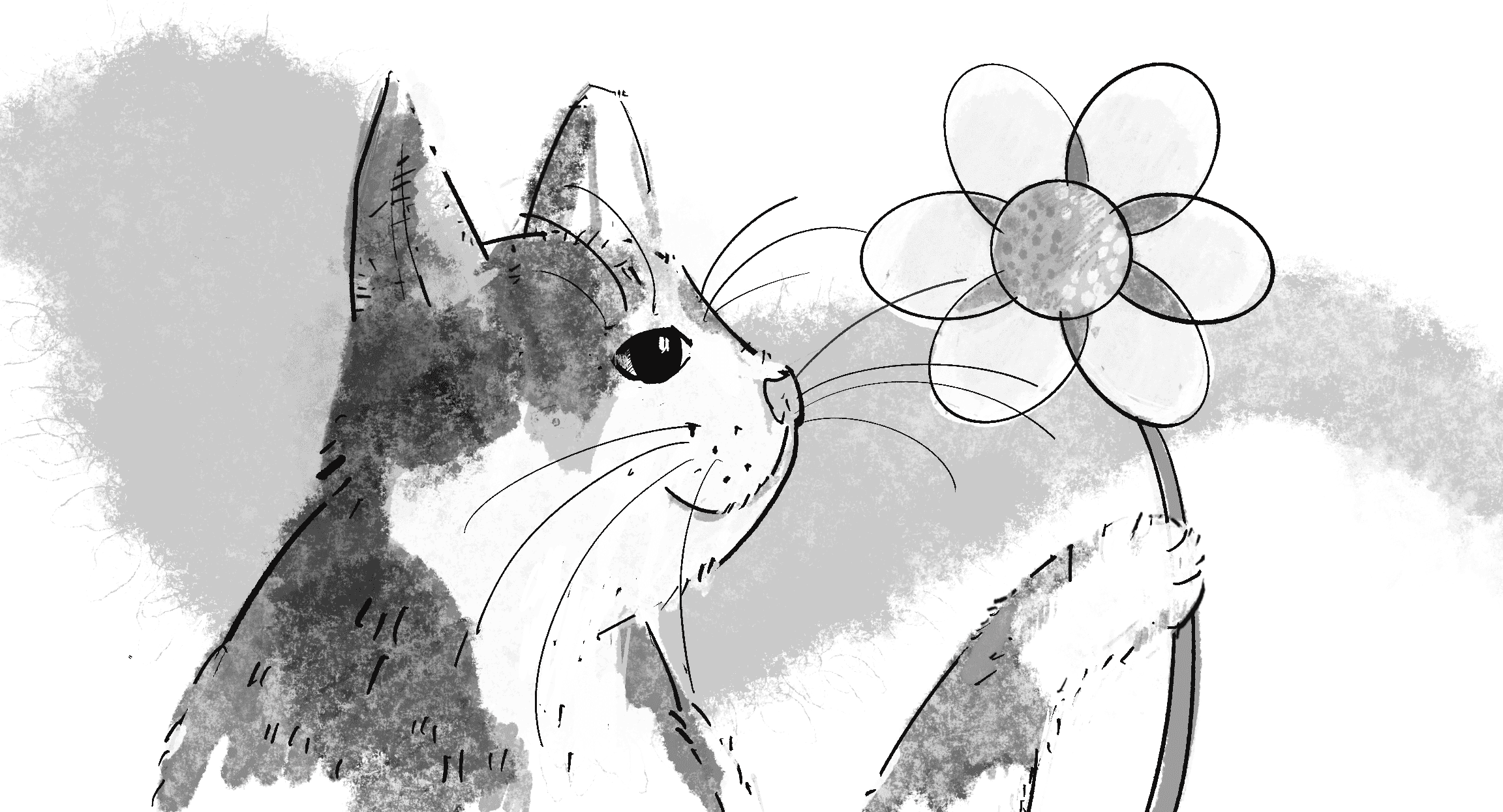
I’d like to build on this idea of the whiskers (or more formally the vibrissae) found in mice, cats, and other mammals. In the real world, animals use their vibrissae to navigate and detect nearby objects, especially in dark or obscured environments (see Figure 11.5). How can I attach whisker-like sensors to my neuroevolutionary-seeking creatures?

I’ll keep the generic class name Creature but think of them now as the amoeba-like bloops from Chapter 9, enhanced with whisker-like sensors that emanate from their center in all directions:

class Creature {

  constructor(x, y) {

    this.position = createVector(x, y);
    this.r = 16;

    this.sensors = [];

    let totalSensors = 8;
    for (let i = 0; i < totalSensors; i++) {

      let angle = map(i, 0, totalSensors, 0, TWO_PI);

      this.sensors[i] = p5.Vector.fromAngle(angle);
      this.sensors[i].setMag(this.r * 1.5);

    }

  }

}

The code creates a series of vectors, each describing the direction and length of one whisker sensor attached to the creature. However, just the vector isn’t enough. I want the sensor to include a value, a numeric representation of what it’s sensing. This value can be thought of as analogous to the intensity of touch. Just as Clawdius the cat’s whiskers might detect a faint touch from a distant object or a stronger push from a closer one, the virtual sensor’s value could range to represent proximity.

Before I go any further, I need to give the creatures something to sense. How about a Food class to describe a circle of deliciousness that the creature wants to find? Each Food object will have a position and a radius:

class Food {

  constructor() {
    this.position = createVector(random(width), random(height));
    this.r = 50;
  }

  show() {

    noStroke();

    fill(0, 100);

    circle(this.position.x, this.position.y, this.r * 2);

  }

}

How can I determine if a creature’s sensor is touching the food? One approach could be to use raycasting. This technique is commonly employed in computer graphics to project straight lines (often representing beams of light) from an origin point in a scene to determine which objects they intersect with. Raycasting is useful for visibility and collision checks, exactly what I’m doing here!

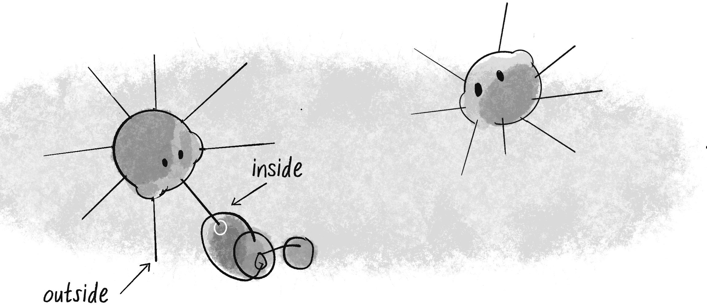
While raycasting would provide a robust solution, it requires more mathematics than I’d like to delve into here. For those interested, an explanation and implementation are available in Coding Challenge #145 on the Coding Train website. For this example, I’ll opt for a more straightforward approach and check whether the endpoint of a sensor lies inside the food circle (see Figure 11.6).

Because I want the sensor to store a value for its sensing along with the sensing algorithm, encapsulating these elements into a Sensor class makes sense:

class Sensor {

  constructor(v) {

    this.v = v.copy();

    this.value = 0;

  }

  sense(position, food) {

    let end = p5.Vector.add(position, this.v);

    let d = end.dist(food.position);

    if (d < food.r) {

      this.value = map(d, 0, food.r, 1, 0);

    } else {

      this.value = 0;

    }

  }

}

Notice that the sensing mechanism gauges the endpoint’s depth within the food’s radius by using the map() function. When the sensor’s endpoint is just touching the outer boundary of the food, value starts at 0. As the endpoint moves closer to the center of the food, value increases, maxing out at 1. If the sensor isn’t touching the food at all, value remains at 0. This gradient of feedback mirrors the varying intensity of touch or pressure in the real world.

Let’s test out this sensor mechanism with a simple example: one bloop (controlled by the mouse) and one piece of food (placed at the center of the canvas). When the sensors touch the food, they light up, and they get brighter as they get closer to the center of the food.

let bloop, food;

function setup() {

  createCanvas(640, 240);

  bloop = new Creature();
  food = new Food();

}

function draw() {

  background(255);

  bloop.position.x = mouseX;
  bloop.position.y = mouseY;

  food.show();
  bloop.show();

  bloop.sense(food);

}

class Creature {

  constructor(x, y) {

    this.position = createVector(x, y);

    this.r = 16;

    this.sensors = [];

    let totalSensors = 15;
    for (let i = 0; i < totalSensors; i++) {
      let a = map(i, 0, totalSensors, 0, TWO_PI);
      let v = p5.Vector.fromAngle(a);
      v.mult(this.r * 2);
      this.sensors[i] = new Sensor(v);
    }

  }

  sense(food) {
    for (let sensor of this.sensors) {
      sensor.sense(this.position, food);
    }

  }

  show() {
    push();
    translate(this.position.x, this.position.y);
    for (let sensor of this.sensors) {
      stroke(0);
      line(0, 0, sensor.v.x, sensor.v.y);
      if (sensor.value > 0) {
        fill(255, sensor.value * 255);
        stroke(0, 100)
        circle(sensor.v.x, sensor.v.y, 8);
      }
    }
    noStroke();
    fill(0);
    circle(0, 0, this.r * 2);
    pop();
  }

}

In the example, the creature’s sensors are drawn as lines from its center. When a sensor detects something (when value is greater than 0), a circle appears. To visualize the strength of the sensor reading, I use value to set its transparency.

Learning from the Sensors

Are you thinking what I’m thinking? What if the values of a creature’s sensors are the inputs to a neural network? Assuming I give the creatures control of their own movements again, I could write a new think() method that processes the sensor values through the neural network brain and outputs a steering force, just as in the last two steering examples:

  think() {

    let inputs = [];
    for (let i = 0; i < this.sensors.length; i++) {
      inputs[i] = this.sensors[i].value;
    }

    let outputs = this.brain.predictSync(inputs);
    let angle = outputs[0].value * TWO_PI;
    let magnitude = outputs[1].value;
    let force = p5.Vector.fromAngle(angle)
    force.setMag(magnitude);
    this.applyForce(force);

  }

The logical next step might be to incorporate all the usual parts of the GA, writing a fitness function (how much food did each creature eat?) and performing selection after a fixed generational time period. But this is a great opportunity to revisit the principles of a continuous ecosystem and aim for a more sophisticated environment and set of potential behaviors for the creatures themselves. Instead of a fixed life span cycle for each generation, I’ll bring back Chapter 9’s health score for each creature. For every cycle through draw() that a creature lives, its health deteriorates a little bit:

class Creature {  

  constructor() {

    /* All of the creature's properties */

    this.health = 100;

  } 

  update() {

    /* The usual updating position, velocity, acceleration */

    this.health -= 0.25;

  }

In draw(), if any bloop’s health drops below 0, that bloop dies and is deleted from the bloops array. And for reproduction, instead of performing the usual crossover and mutation all at once, each bloop (with a health greater than 0) will have a 0.1 percent chance of reproducing:

  function draw() {

    for (let i = bloops.length - 1; i >= 0; i--) {

      if (bloops[i].health < 0) {

        bloops.splice(i, 1);

      } else if (random(1) < 0.001) {

        let child = bloops[i].reproduce();

        bloops.push(child);

      }

    }

  }

In reproduce(), I’ll use the copy() method (cloning) instead of the crossover() method (mating), with a higher-than-usual mutation rate to help introduce variation. (I encourage you to consider ways to incorporate crossover instead.) Here’s the code:

  reproduce() {

    let brain = this.brain.copy();
    brain.mutate(0.1);

    return new Creature(this.position.x, this.position.y, brain);

  }

For this to work, some bloops should live longer than others. By consuming food, their health increases, giving them extra time to reproduce. I’ll manage this in an eat() method of the Creature class:

  eat(food) {

    let d = p5.Vector.dist(this.position, food.position);
    if (d < this.r + food.r) {
      this.health += 0.5;
    }

  }

Is this enough for the system to evolve and find its equilibrium? I could dive deeper, tweaking parameters and behaviors in pursuit of the ultimate evolutionary system. The allure of this infinite rabbit hole is one I cannot easily escape, but I’ll explore it on my own time. For the purpose of this book, I invite you to run the example, experiment, and draw your own conclusions.

let bloops = [];

let food = [];

function setup() {

  createCanvas(640, 240);

  for (let i = 0; i < 20; i++) {

    bloops[i] = new Creature(random(width), random(height));

  }

  for (let i = 0; i < 8; i++) {

    food[i] = new Food();

  }

}

function draw() {

  background(255);

  for (let i = bloops.length - 1; i >= 0; i--) {

    bloops[i].think();

    bloops[i].eat();

    bloops[i].update();

    bloops[i].borders();

    if (bloops[i].health < 0) {

      bloops.splice(i, 1);

    } else if (random(1) < 0.001) {

      let child = bloops[i].reproduce();

      bloops.push(child);

    }

  }

  for (let treat of food) {

    treat.show();

  }

  for (let bloop of bloops) {

    bloop.show();

  }

}

The final example also includes a few additional features that you’ll find in the accompanying online code, such as an array of food that shrinks as it gets eaten (respawning when it’s depleted). Additionally, the bloops shrink as their health deteriorates.

The Ecosystem Project

Try incorporating the concept of a brain into the creatures in your world!

• Can different creatures have different goals and incentives? Are some searching for food while others seek different resources? What about creatures avoiding dangers like predators or poisons?
• What are each creature’s inputs and outputs?
• How do the creatures perceive? Do they see everything or have limits based on sensors?
• What strategies can you employ to establish and maintain balance in your ecosystem?

The End

If you’re still reading, thank you! You’ve reached the end of the book. But for as much material as this book contains, I’ve barely scratched the surface of the physical world we inhabit and of techniques for simulating it. I intend for this book to live as an ongoing project, and I hope to continue adding new tutorials and examples to the book’s website, as well as expand and update the accompanying video tutorials at the Coding Train website.

Your feedback is truly appreciated, so please get in touch via email at daniel@shiffman.net or by contributing to the GitHub repository, in keeping with the open source spirit of the project. Share your work. Stay in touch. Let’s be two with nature.