Chapter 3: Oscillation
Trigonometry is a sine of the times.
—Anonymous


Bridget Riley, a celebrated British artist, was a driving force behind the Op Art movement of the 1960s. Her work features geometric patterns that challenge the viewer’s perceptions and evoke feelings of movement or vibration. Her 1974 piece Gala showcases a series of curvilinear forms that ripple across the canvas, evoking the natural rhythm of the sine wave.
In Chapters 1 and 2, I carefully worked out an object-oriented structure to animate a shape in a p5.js canvas, using a vector to represent position, velocity, and acceleration driven by forces in the environment. I could move straight from here into topics such as particle systems, steering forces, group behaviors, and more. However, doing so would mean skipping a fundamental aspect of motion in the natural world: oscillation, or the back-and-forth movement of an object around a central point or position.
To model oscillation, you need to understand a little bit about trigonometry, the mathematics of triangles. Learning some trig will give you new tools to generate patterns and create new motion behaviors in a p5.js sketch. You’ll learn to harness angular velocity and acceleration to spin objects as they move. You’ll be able to use the sine and cosine functions to model nice ease-in, ease-out wave patterns. You’ll also learn to calculate the more complex forces at play in situations that involve angles, such as a pendulum swinging or a box sliding down an incline.
I’ll start with the basics of working with angles in p5.js, then cover several aspects of trigonometry. In the end, I’ll connect trigonometry with what you learned about forces in Chapter 2. This chapter’s content will pave the way for more sophisticated examples that require trig later in this book.
Angles

Before going any further, I need to make sure you understand how the concept of an angle fits into creative coding in p5.js. If you have experience with p5.js, you’ve undoubtedly encountered this issue while using the rotate() function to rotate and spin objects. You’re most likely to be familiar with the concept of an angle as measured in degrees (see Figure 3.1).


A full rotation goes from 0 to 360 degrees, and 90 degrees (a right angle) is one-fourth of 360, shown in Figure 3.1 as two perpendicular lines.
Angles are commonly used in computer graphics to specify a rotation for a shape. For example, the square in Figure 3.2 is rotated 45 degrees around its center.

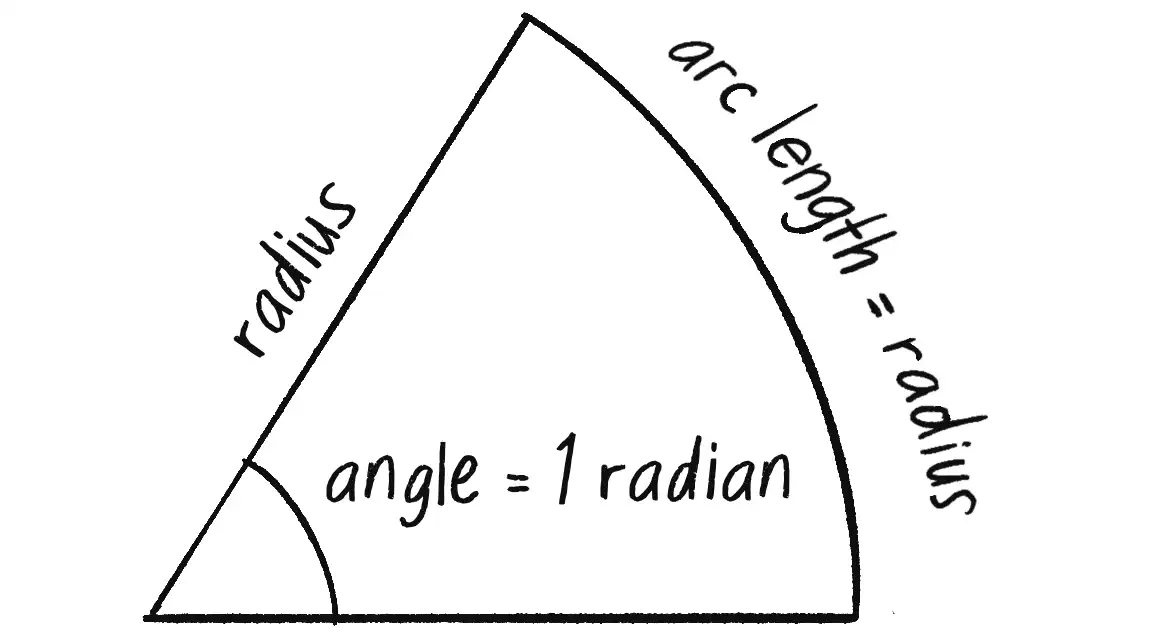
The catch is that, by default, p5.js measures angles not in degrees but in radians. This alternative unit of measurement is defined by the ratio of the length of the arc of a circle (a segment of the circle’s circumference) to the radius of that circle. One radian is the angle at which that ratio equals 1 (see Figure 3.3). A full circle (360 degrees) is equivalent to radians, 180 degrees is equivalent to radians, and 90 degrees is equivalent to radians.
The formula to convert from degrees to radians is as follows:
Thankfully, if you prefer to think of angles in degrees, you can call angleMode(DEGREES), or you can use the convenience function radians() to convert values from degrees to radians. The constants PI, TWO_PI, and HALF_PI are also available (equivalent to 180, 360, and 90 degrees, respectively). For example, here are two ways in p5.js to rotate a shape by 60 degrees:
let angle = 60;
rotate(radians(angle));
angleMode(DEGREES);
rotate(angle);
What Is Pi?
The mathematical constant pi (or the Greek letter ) is a real number defined as the ratio of a circle’s circumference (the distance around the outside of the circle) to its diameter (a straight line that passes through the circle’s center). It’s equal to approximately 3.14159 and can be accessed in p5.js with the built-in PI variable.
While degrees can be useful, for the purposes of this book, I’ll be working with radians because they’re the standard unit of measurement across many programming languages and graphics environments. If they’re new to you, this is a good opportunity to practice! Additionally, if you aren’t familiar with the way rotation is implemented in p5.js, I recommend watching my Coding Train video series on transformations in p5.js.
Exercise 3.1
Rotate a baton-like object around its center by using translate() and rotate().
Angular Motion

Another term for rotation is angular motion—that is, motion about an angle. Just as linear motion can be described in terms of velocity—the rate at which an object’s position changes over time—angular motion can be described in terms of angular velocity—the rate at which an object’s angle changes over time. By extension, angular acceleration describes changes in an object’s angular velocity.
Luckily, you already have all the math you need to understand angular motion. Remember the stuff I dedicated almost all of Chapters 1 and 2 to explaining?
You can apply exactly the same logic to a rotating object:
In fact, these angular motion formulas are simpler than their linear motion equivalents since the angle here is a scalar quantity (a single number), not a vector! This is because in 2D space, there’s one axis of rotation; in 3D space, the angle would become a vector. (Note that in most contexts, these formulas would include a multiplication by the change in time, referred to as delta time. I’m assuming a delta time of 1 that corresponds to one frame of animation in p5.js.)
Using the answer from Exercise 3.1, let’s say you wanted to rotate a baton in p5.js by a certain angle. Originally, the code might have read as follows:
translate(width / 2, height / 2);
rotate(angle);
line(-60, 0, 60, 0);
circle(60, 0, 16);
circle(-60, 0, 16);
angle = angle + 0.1;
Adding in the principles of angular motion, I can instead write the following example (the solution to Exercise 3.1).
Example 3.1: Angular Motion Using rotate()
let angle = 0;
Position
let angleVelocity = 0;
Velocity
let angleAcceleration = 0.0001;
Acceleration
function setup() {
createCanvas(640, 240);
}
function draw() {
background(255);
translate(width / 2, height / 2);
rotate(angle);
Rotate according to that angle.
stroke(0);
fill(127);
line(-60, 0, 60, 0);
circle(60, 0, 16);
circle(-60, 0, 16);
angleVelocity += angleAcceleration;
Angular equivalent of velocity.add(acceleration)
angle += angleVelocity;
Angular equivalent of position.add(velocity)
}
Instead of incrementing angle by a fixed amount to steadily rotate the baton, for every frame I add angleAcceleration to angleVelocity, then add angleVelocity to angle. As a result, the baton starts with no rotation and then spins faster and faster as the angular velocity accelerates.
Exercise 3.2
Add an interaction to the spinning baton. How can you control the acceleration with the mouse? Can you introduce the idea of drag, decreasing the angular velocity over time so the baton eventually comes to rest?
The logical next step is to incorporate this idea of angular motion into the Mover class. First, I need to add some variables to the class’s constructor:
class Mover {
constructor() {
this.position = createVector(width / 2, height / 2);
this.velocity = createVector(0, 0);
this.acceleration = createVector(0, 0);
this.mass = 1.0;
    this.angle = 0;
    this.angleVelocity = 0;
    this.angleAcceleration = 0;
Variables for angular motion
}
Then, in update(), the mover’s position and angle are updated according to the algorithm I just demonstrated:
update() {
    this.velocity.add(this.acceleration);
    this.position.add(this.velocity);
Regular old-fashioned motion
    this.angleVelocity += this.angleAcceleration;
    this.angle += this.angleVelocity;
Newfangled angular motion
this.acceleration.mult(0);
}
Of course, for any of this to matter, I also need to rotate the object when drawing it in the show() method. (I’ll add a line from the center to the edge of the circle so that rotation is visible. You could also draw the object as a shape other than a circle.)
show() {
stroke(0);
fill(175, 200);
push();
Use push() to save the current state so the rotation of this shape doesn’t affect the rest of the world.
translate(this.position.x, this.position.y);
Set the origin at the shape’s position.
rotate(this.angle);
Rotate by the angle.
circle(0, 0, this.radius * 2);
line(0, 0, this.radius, 0);
pop();
Use pop() to restore the previous state after rotation is complete.
}
At this point, if you were to actually go ahead and create a Mover object, you wouldn’t see it behave any differently. This is because the angular acceleration is initialized to zero (this.angleAcceleration = 0;). For the object to rotate, it needs a nonzero acceleration! Certainly, one option is to hardcode a number in the constructor:
this.angleAcceleration = 0.01;
You can produce a more interesting result, however, by dynamically assigning an angular acceleration in the update() method according to forces in the environment. This could be my cue to start researching the physics of angular acceleration based on the concepts of torque and moment of inertia, but at this stage, that level of simulation would be a bit of a rabbit hole. (I’ll cover modeling angular acceleration with a pendulum in more detail in “The Pendulum”, as well as look at how third-party physics libraries realistically model rotational motion in Chapter 6.)
Instead, a quick-and-dirty solution that yields creative results will suffice. A reasonable approach is to calculate angular acceleration as a function of the object’s linear acceleration, its rate of change of velocity along a path vector, as opposed to its rotation. Here’s an example:
this.angleAcceleration = this.acceleration.x;
Use the x-component of the object’s linear acceleration to calculate angular acceleration.
Yes, this is arbitrary, but it does do something. If the object is accelerating to the right, its angular rotation accelerates in a clockwise direction; acceleration to the left results in a counterclockwise rotation. Of course, it’s important to think about scale in this case. The value of the acceleration vector’s x component might be too large, causing the object to spin in a way that looks ridiculous or unrealistic. You might even notice a visual illusion called the wagon wheel effect: an object appears to be rotating more slowly or even in the opposite direction because of the large changes between each frame of animation.
Dividing the x component by a value, or perhaps constraining the angular velocity to a reasonable range, could really help. Here’s the entire update() function with these tweaks added.
Example 3.2: Forces with (Arbitrary) Angular Motion
update() {
this.velocity.add(this.acceleration);
this.position.add(this.velocity);
this.angleAcceleration = this.acceleration.x / 10.0;
Calculate angular acceleration according to acceleration’s x-component.
this.angleVelocity += this.angleAcceleration;
this.angleVelocity = constrain(this.angleVelocity, -0.1, 0.1);
Use constrain() to ensure that angular velocity doesn’t spin out of control.
this.angle += this.angleVelocity;
this.acceleration.mult(0);
}
Notice that I’ve used multiple strategies to keep the object from spinning out of control. First, I divide acceleration.x by 10 before assigning it to angleAcceleration. Then, for good measure, I also use constrain() to confine angleVelocity to the range (–0.1, 0.1).
Exercise 3.3
Step 1: Create a simulation of objects being shot out of a cannon. Each object should experience a sudden force when shot (just once) as well as gravity (always present).
Step 2: Add rotation to the object to model its spin as it’s shot from the cannon. How realistic can you make it look?
Trigonometry Functions
I think I’m ready to reveal the secret of trigonometry. I’ve discussed angles, I’ve spun a baton. Now it’s time for . . . wait for it . . . sohcahtoa. Yes, sohcahtoa! This seemingly nonsensical word is actually the foundation for much of computer graphics work. A basic understanding of trigonometry is essential if you want to calculate angles, figure out distances between points, and work with circles, arcs, or lines. And sohcahtoa is a mnemonic device (albeit a somewhat absurd one) for remembering the meanings of the trigonometric functions sine, cosine, and tangent. It references the sides of a right triangle, as shown in Figure 3.4.

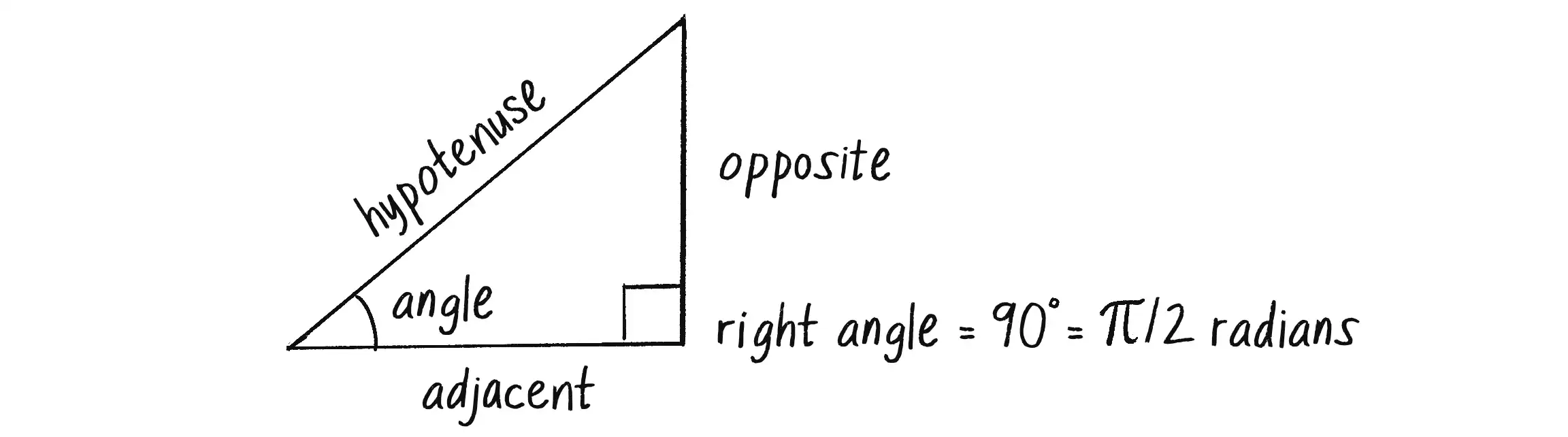
Take one of the non-right angles in the triangle. The adjacent side is the one touching that angle, the opposite side is the one not touching that angle, and the hypotenuse is the side opposite the right angle. Sohcahtoa tells you how to calculate the angle’s trigonometric functions in terms of the lengths of these sides:
- soh:
- cah:
- toa:
Take a look at Figure 3.4 again. You don’t need to memorize it, but see if you feel comfortable with it. Try redrawing it yourself. Next, let’s look at it in a slightly different way (see Figure 3.5).

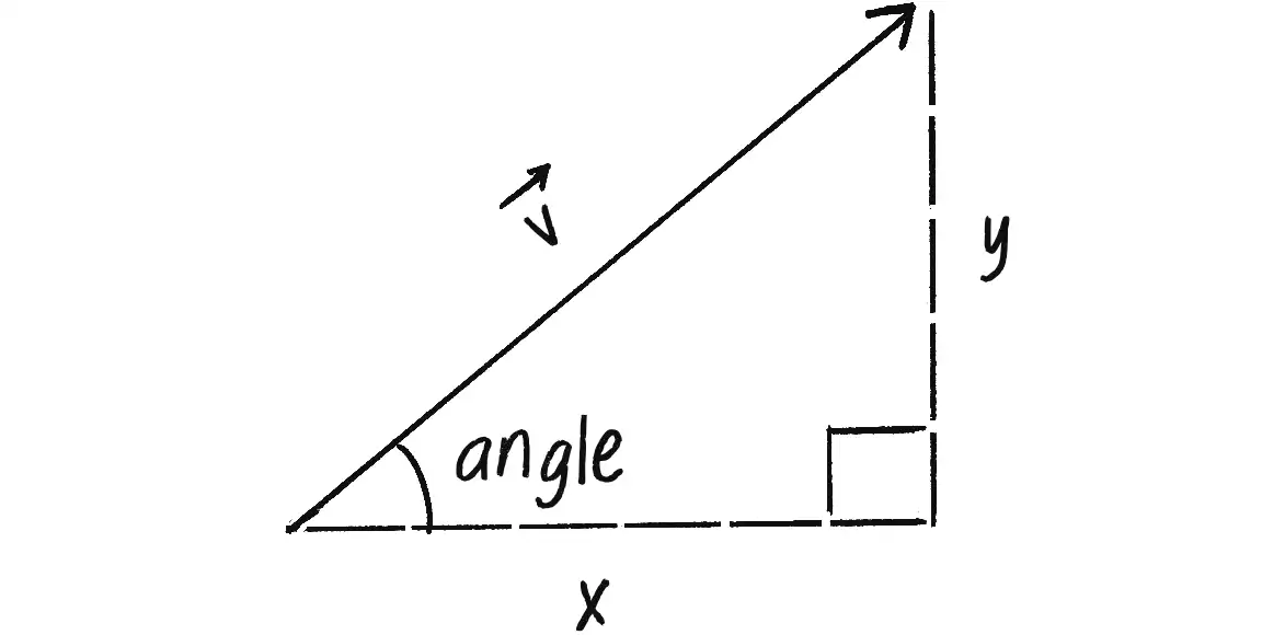
See how a right triangle is created from the vector ? The vector arrow is the hypotenuse, and the components of the vector (x and y) are the sides of the triangle. The angle is an additional means for specifying the vector’s direction (or heading). Viewed in this way, the trigonometric functions establish a relationship between the components of a vector and its direction + magnitude. As such, trigonometry will prove very useful throughout this book. To illustrate this, let’s look at an example that requires the tangent function.
Pointing in the Direction of Movement

Think all the way back to Example 1.10, which featured a Mover object accelerating toward the mouse (Figure 3.6).
You might notice that almost all the shapes I’ve been drawing so far have been circles. This is convenient for several reasons, one of which is that using circles allows me to avoid the question of rotation. Rotate a circle and, well, it looks exactly the same. Nevertheless, there comes a time in all motion programmers’ lives when they want to move something around onscreen that isn’t shaped like a circle. Perhaps it’s an ant, or a car, or a spaceship. To look realistic, that object should point in its direction of movement.
When I say “point in its direction of movement,” what I really mean is “rotate according to its velocity vector.” Velocity is a vector, with an x- and y-component, but to rotate in p5.js, you need one number, an angle. Let’s look at the trigonometry diagram once more, this time focused on an object’s velocity vector (Figure 3.7).

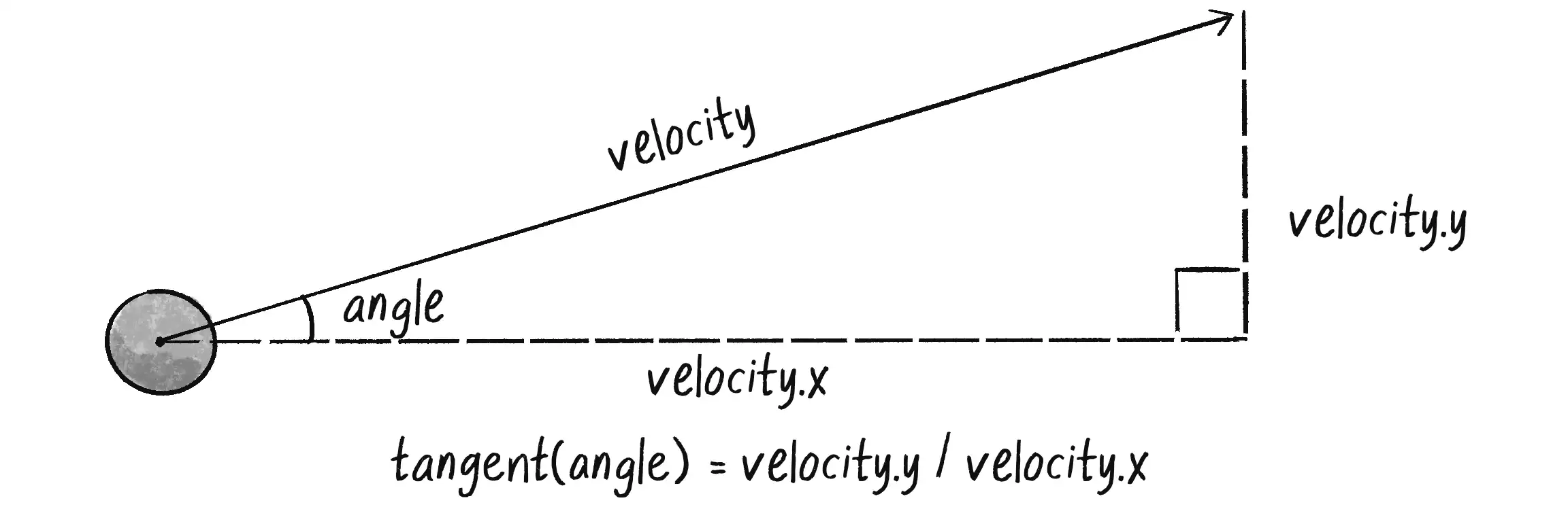
The vector’s x- and y-components are related to its angle through the tangent function. Using the toa in sohcahtoa, I can write the relationship as follows:
The problem here is that while I know the x- and y-components of the velocity vector, I don’t know the angle of its direction. I have to solve for that angle. This is where another function known as the inverse tangent, or arctangent (arctan or atan, for short), comes in. (There are also inverse sine and inverse cosine functions, called arcsine and arccosine, respectively.)
If the tangent of value a equals value b, then the inverse tangent of b equals a. For example:
| If | |
| then |
See how one is the inverse of the other? This allows me to solve for the vector’s angle:
| If | |
| then |
Now that I have the formula, let’s see where it should go in the Mover class’s show() method to make the mover (now drawn as a rectangle) point in its direction of motion. Note that in p5.js, the function for inverse tangent is atan():
show() {
let angle = atan(this.velocity.y / this.velocity.x);
Solve for the angle by using atan().
stroke(0);
fill(175);
push();
rectMode(CENTER);
translate(this.position.x, this.position.y);
rotate(angle);
Rotate according to that angle.
rect(0, 0, 30, 10);
pop();
}


This code is pretty darn close and almost works. There’s a big problem, though. Consider the two velocity vectors depicted in Figure 3.8.
Though superficially similar, the two vectors point in quite different directions—opposite directions, in fact! In spite of this, look at what happens if I apply the inverse tangent formula to solve for the angle of each vector:
I get the same angle! That can’t be right, though, since the vectors are pointing in opposite directions. It turns out this is a pretty common problem in computer graphics. I could use atan() along with conditional statements to account for positive/negative scenarios, but p5.js (along with most programming environments) has a helpful function called atan2() that resolves the issue for me.
Example 3.3: Pointing in the Direction of Motion
show() {
let angle = atan2(this.velocity.y, this.velocity.x);
Use atan2() to account for all possible directions.
push();
rectMode(CENTER);
translate(this.position.x, this.position.y);
rotate(angle);
Rotate according to that angle.
rect(0, 0, 30, 10);
pop();
}
To simplify this even further, the p5.Vector class provides a method called heading(), which takes care of calling atan2() and returns the 2D direction angle, in radians, for any p5.Vector:
let angle = this.velocity.heading();
The easiest way to do this!
With heading(), it turns out you don’t actually need to implement the trigonometry functions in your code, but understanding how they’re all working is still helpful.
Exercise 3.4
Create a simulation of a vehicle that you can drive around the screen by using the arrow keys: the left arrow accelerates the car to the left, and the right arrow accelerates to the right. The car should point in the direction in which it’s currently moving.
Polar vs. Cartesian Coordinates

Anytime you draw a shape in p5.js, you have to specify a pixel position, a set of x- and y-coordinates. These are known as Cartesian coordinates, named for René Descartes, the French mathematician who developed the ideas behind Cartesian space.
Another useful coordinate system, known as polar coordinates, describes a point in space as a distance from the origin (like the radius of a circle) and an angle of rotation around the origin (usually called , the Greek letter theta). Thinking in terms of vectors, a Cartesian coordinate describes a vector’s x- and y-components, whereas a polar coordinate describes a vector’s magnitude (length) and direction (angle).
When working in p5.js, you may find it more convenient to think in polar coordinates, especially when creating sketches that involve rotational or circular movements. However, p5.js’s drawing functions understand only (x, y) Cartesian coordinates. Happily for you, trigonometry holds the key to converting back and forth between polar and Cartesian (see Figure 3.9). This allows you to design with whatever coordinate system you have in mind, while always drawing using Cartesian coordinates.

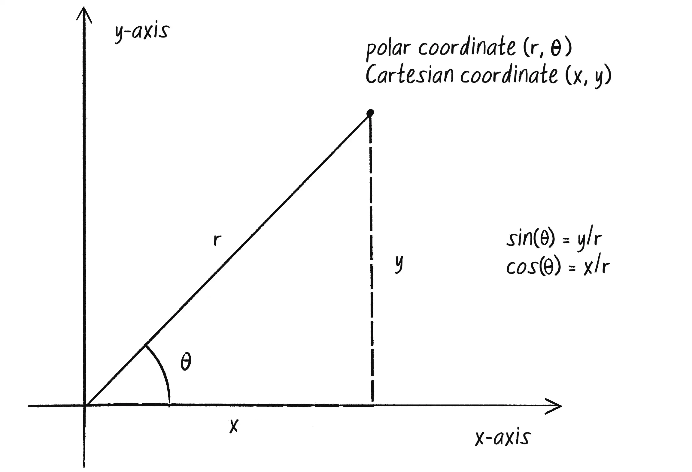
theta as a variable name when referring to an angle in p5.js.For example, given a polar coordinate with a radius of 75 pixels and an angle () of 45 degrees (or radians), the Cartesian x and y can be computed as follows:
The functions for sine and cosine in p5.js are sin() and cos(), respectively. Each takes one argument, a number representing an angle in radians. These formulas can thus be coded as follows:
let r = 75;
let theta = PI / 4;
let x = r * cos(theta);
let y = r * sin(theta);
Convert from polar (r, theta) to Cartesian (x, y).
This type of conversion can be useful in certain applications. For instance, moving a shape along a circular path using Cartesian coordinates isn’t so easy. However, with polar coordinates, it’s simple: just increment the angle! Here’s how it’s done with global r and theta variables.
Example 3.4: Polar to Cartesian
let r;
let theta;
function setup() {
createCanvas(640, 240);
  r = height * 0.45;
  theta = 0;
Initialize all values.
}
function draw() {
background(255);
translate(width / 2, height / 2);
Translate the origin point to the center of the screen.
  let x = r * cos(theta);
  let y = r * sin(theta);
Polar coordinates (r, theta) are converted to Cartesian (x, y) for use in the circle() function.
fill(127);
stroke(0);
line(0, 0, x, y);
circle(x, y, 48);
theta += 0.02;
Increase the angle over time.
}
Polar-to-Cartesian conversion is common enough that p5.js includes a handy function to take care of it for you. It’s included as a static method of the p5.Vector class called fromAngle(). It takes an angle in radians and creates a unit vector in Cartesian space that points in the direction specified by the angle. Here’s how that would look in Example 3.4:
let position = p5.Vector.fromAngle(theta);
Create a unit vector pointing in the direction of an angle.
position.mult(r);
To complete polar-to-Cartesian conversion, scale position by r.
circle(position.x, position.y, 48);
Draw the circle by using the x- and y-components of the vector.
Are you amazed yet? I’ve demonstrated some pretty great uses of tangent (for finding the angle of a vector) and sine and cosine (for converting from polar to Cartesian coordinates). I could stop right here and be satisfied. But I’m not going to. This is only the beginning. As I’ll show you next, what sine and cosine can do for you goes beyond mathematical formulas and right triangles.
Exercise 3.5
Using Example 3.4 as a basis, draw a spiral path. Start in the center and move outward. Note that this can be done by changing only one line of code and adding one line of code!
Exercise 3.6
Simulate the spaceship in the game Asteroids. In case you aren’t familiar with Asteroids, here’s a brief description: A spaceship (represented as a triangle) floats in 2D space. The left arrow key turns the spaceship counterclockwise; the right arrow key turns it clockwise. The Z key applies a thrust force in the direction the spaceship is pointing.
Properties of Oscillation

Take a look at the graph of the sine function in Figure 3.10, where y = sin(x).

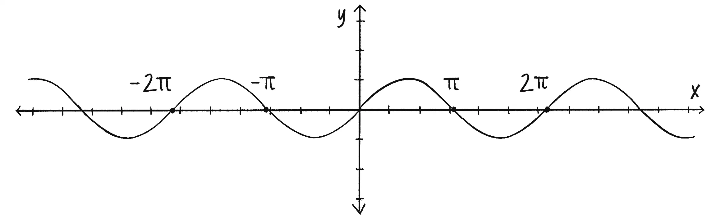
The output of the sine function is a smooth curve alternating between –1 and 1, also known as a sine wave. This behavior, a periodic movement between two points, is the oscillation I mentioned at the start of the chapter. Plucking a guitar string, swinging a pendulum, bouncing on a pogo stick—all are examples of oscillating motion that can be modeled using the sine function.
In a p5.js sketch, you can simulate oscillation by assigning the output of the sine function to an object’s position. I’ll begin with a basic scenario: I want a circle to oscillate between the left side and the right side of a canvas (Figure 3.11).
This pattern of oscillating back and forth around a central point is known as simple harmonic motion (or, to be fancier, the periodic sinusoidal oscillation of an object). The code to achieve it is remarkably simple, but before I get into it, I’d like to introduce some of the key terminology related to oscillation (and waves).
When a moving object exhibits simple harmonic motion, its position (in this case, the x-position) can be expressed as a function of time, with the following two elements:
- Amplitude: The distance from the center of motion to either extreme
- Period: The duration (time) for one complete cycle of motion
To understand these terms, look again at the graph of the sine function in Figure 3.10. The curve never rises above 1 or below –1 along the y-axis, so the sine function has an amplitude of 1. Meanwhile, the wave pattern of the curve repeats every units along the x-axis, so the sine function’s period is . (By convention, the units here are radians, since the input value to the sine function is customarily an angle measured in radians.)
So much for the amplitude and period of an abstract sine function, but what are amplitude and period in the p5.js world of an oscillating circle? Well, amplitude can be measured rather easily in pixels. For example, if the canvas is 200 pixels wide, I might choose to oscillate around the center of the canvas, going between 100 pixels right of center and 100 pixels left of center. In other words, the amplitude is 100 pixels.
let amplitude = 100;
The amplitude is measured in pixels.
The period is the amount of time for one complete cycle of an oscillation. However, in a p5.js sketch, what does time really mean? In theory, I could say I want the circle to oscillate every three seconds, then come up with an elaborate algorithm for moving the object according to real-world time, using millis() to track the passage of milliseconds. For what I’m trying to accomplish here, however, real-world time isn’t necessary. The more useful measure of time in p5.js is the number of frames that have elapsed, available through the built-in frameCount variable. Do I want the oscillating motion to repeat every 30 frames? Every 50 frames? For now, how about a period of 120 frames:
let period = 120;
The period is measured in frames (the unit of time for animation).
Once I have the amplitude and period, it’s time to write a formula to calculate the circle’s x-position as a function of time (the current frame count):
let x = amplitude * sin(TWO_PI * frameCount / period);
amplitude and period are my own variables; frameCount is built into p5.js.
Think about what’s going on here. First, whatever value the sin() function returns is multiplied by amplitude. As you saw in Figure 3.10, the output of the sine function oscillates between –1 and 1. Multiplying that value by my chosen amplitude—call it a—gives me the desired result: a value that oscillates between –a and a. (This is also a place where you could use p5.js’s map() function to map the output of sin() to a custom range.)
Now, think about what’s inside the sin() function:
TWO_PI * frameCount / period
What’s going on here? Start with what you know. I’ve explained that sine has a period of , meaning it will start at 0 and repeat at , , , and so on. If my desired period of oscillation is 120 frames, I want the circle to be in the same position when frameCount is at 120 frames, 240 frames, 360 frames, and so on. Here, frameCount is the only value changing over time; it starts at 0 and counts upward. Let’s take a look at what the formula yields as frameCount increases.
frameCount | frameCount / period | TWO_PI * frameCount / period |
|---|---|---|
| 0 | 0 | 0 |
| 60 | 0.5 | |
| 120 | 1 | |
| 240 | 2 | |
| . . . | . . . | . . . |
Dividing frameCount by period tells me the number of cycles that have been completed. (Is the wave halfway through the first cycle? Have two cycles completed?) Multiplying that number by TWO_PI, I get the desired result, an appropriate input to the sin() function, since TWO_PI is the value required for sine (or cosine) to complete one full cycle.
Putting it together, here’s an example that oscillates the x position of a circle with an amplitude of 100 pixels and a period of 120 frames.
Example 3.5: Simple Harmonic Motion I
function setup() {
createCanvas(640, 240);
}
function draw() {
background(255);
let period = 120;
let amplitude = 200;
let x = amplitude * sin(TWO_PI * frameCount / period);
Calculate the horizontal position according to the formula for simple harmonic motion.
stroke(0);
fill(127);
translate(width / 2, height / 2);
line(0, 0, x, 0);
circle(x, 0, 48);
}
Before moving on, I would be remiss not to mention frequency, the number of cycles of an oscillation per time unit. Frequency is the inverse of the period—that is, 1 divided by the period. For example, if the period is 120 frames, only 1/120th of a cycle is completed in 1 frame, and so the frequency is 1/120. In Example 3.5, I chose to define the rate of oscillation in terms of the period, and therefore I didn’t need a variable for frequency. Sometimes, however, thinking in terms of frequency rather than period is more useful.
Exercise 3.7
Using the sine function, create a simulation of a weight (sometimes referred to as a bob) that hangs from a spring from the top of the window. Use the map() function to calculate the vertical position of the bob. In “Spring Forces”, I’ll demonstrate how to create this same simulation by modeling the forces of a spring according to Hooke’s law.
Oscillation with Angular Velocity
An understanding of oscillation, amplitude, and period (or frequency) can be essential in the course of simulating real-world behaviors. However, there’s a slightly easier way to implement the simple harmonic motion from Example 3.5, one that achieves the same result with fewer variables. Take one more look at the oscillation formula:
let x = amplitude * sin(TWO_PI * frameCount / period);
Now I’ll rewrite it in a slightly different way:
let x = amplitude * sin( some value that increments slowly );
If you care about precisely defining the period of oscillation in terms of frames of animation, you might need the formula as I first wrote it. If you don’t care about the exact period, however—for example, if you’ll be choosing it randomly—all you really need inside the sin() function is a value that increments slowly enough for the object’s motion to appear smooth from one frame to the next. Every time this value ticks past a multiple of , the object will have completed one cycle of oscillation.
This technique mirrors what I did with Perlin noise in Chapter 0. In that case, I incremented an offset variable (which I called t or xoff) to sample various outputs from the noise() function, creating a smooth transition of values. Now, I’m going to increment a value (I’ll call it angle) that’s fed into the sin() function. The difference is that the output from sin() is a smoothly repeating sine wave, without any randomness.
You might be wondering why I refer to the incrementing value as angle, given that the object has no visible rotation. The term angle is used because the value is passed into the sin() function, and angles are the traditional inputs to trigonometric functions. With this in mind, I can reintroduce the concept of angular velocity (and acceleration) to rewrite the example to calculate the x position in terms of a changing angle. I’ll assume these global variables:
let angle = 0;
let angleVelocity = 0.05;
I can then write this:
function draw() {
angle += angleVelocity;
let x = amplitude * sin(angle);
}
Here angle is my “value that increments slowly,” and the amount it slowly increments by is angleVelocity.
Example 3.6: Simple Harmonic Motion II
let angle = 0;
let angleVelocity = 0.05;
function setup() {
createCanvas(640, 240);
}
function draw() {
background(255);
let amplitude = 200;
let x = amplitude * sin(angle);
angle += angleVelocity;
Use the concept of angular velocity to increment an angle variable.
translate(width / 2, height / 2);
stroke(0);
fill(127);
line(0, 0, x, 0);
circle(x, 0, 48);
}
Just because I’m not referencing the period directly doesn’t mean that I’ve eliminated the concept. After all, the greater the angular velocity, the faster the circle will oscillate (and therefore the shorter the period). In fact, the period is the number of frames it takes for angle to increment by . Since the amount angle increments is controlled by the angular velocity, I can calculate the period as follows:
To illustrate the power of thinking of oscillation in terms of angular velocity, I’ll expand the example a bit more by creating an Oscillator class whose objects can oscillate independently along both the x-axis (as before) and the y-axis. The class will need two angles, two angular velocities, and two amplitudes (one for each axis).
This is a perfect opportunity to use createVector() to package each pair of values together! Unlike previous vectors, the values in these vectors won’t be sets of Cartesian coordinates. Nevertheless, the p5.Vector class provides a convenient way to manage pairs of values—in this case, pairs of angles (and their associated velocities, accelerations, and so on).
Example 3.7: Oscillator Objects
class Oscillator {
constructor() {
this.angle = createVector(0, 0);
Use a p5.Vector to track two angles!
this.angleVelocity = createVector(random(-0.05, 0.05), random(-0.05, 0.05));
this.amplitude = createVector(random(20, width / 2), random(20, height / 2));
Random velocities and amplitudes
}
update() {
this.angle.add(this.angleVelocity);
}
show() {
let x = sin(this.angle.x) * this.amplitude.x;
Oscillating on the x-axis
let y = sin(this.angle.y) * this.amplitude.y;
Oscillating on the y-axis
push();
translate(width / 2, height / 2);
stroke(0);
fill(127);
    line(0, 0, x, y);
    circle(x, y, 32);
    pop();
Draw the oscillator as a line connecting a circle.
}
}
To better understand the Oscillator class, it might be helpful to focus on the movement of a single oscillator in the animation. First, observe its horizontal movement. You’ll notice that it oscillates regularly back and forth along the x-axis. Switching your focus to its vertical movement, you’ll see it oscillating up and down along the y-axis. Each oscillator has its own distinct rhythm, given the random initialization of its angle, angular velocity, and amplitude.
The key is to recognize that the x and y properties of the p5.Vector objects this.angle, this.angleVelocity, and this.amplitude aren’t tied to spatial vectors anymore. Instead, they’re used to store the respective properties for two separate oscillations (one along the x-axis, one along the y-axis). Ultimately, these oscillations are manifested spatially when x and y are calculated in the show() method, mapping the oscillations onto the positions of the object.
Exercise 3.8
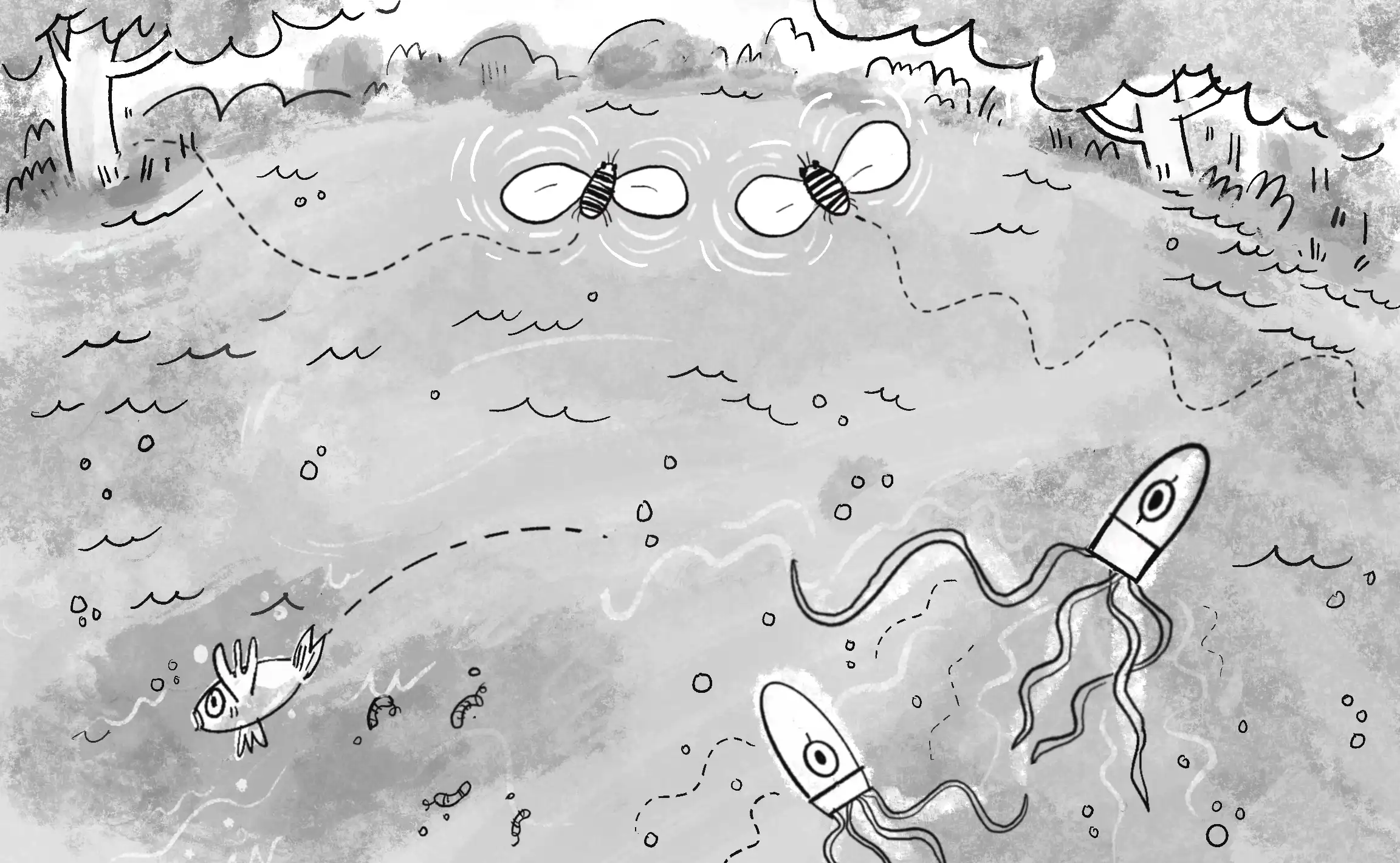
Try initializing each Oscillator object with velocities and amplitudes that aren’t random to create some sort of regular pattern. Can you make the oscillators appear to be the legs of an insect-like creature?
Exercise 3.9
Incorporate angular acceleration into the Oscillator object.
Waves

Imagine a single circle oscillating up and down according to the sine function. This is the equivalent of simulating a single point along the x-axis of a wave. With a little panache and a for loop, you can animate the entire wave by placing a series of oscillating circles next to one another (Figure 3.12).
You could use this wavy pattern to design the body or appendages of a creature, or to simulate a soft surface (such as water). Let’s dive into how the code for this sketch works.
Here, the same concepts of amplitude (the wave’s height) and period (the wave’s duration) come into play. However, when drawing the entire wave, the term period shifts its meaning from representing time to describing the width (in pixels) of a full wave cycle. The term for the spatial period (as opposed to the temporal period) of a wave is wavelength—the distance a wave travels to complete one full oscillation cycle. And just as with the previous oscillation example, you have the choice of computing the wave pattern according to a precise wavelength or by arbitrarily incrementing the angle value (delta angle) for each spot on the wave.
I’ll go with the simpler case, incrementing the angle. I know I need three variables: an angle, a delta angle (analogous to the previous angular velocity), and an amplitude:
let angle = 0;
let deltaAngle = 0.2;
let amplitude = 100;
Then I’m going to loop through all the x values for each point on the wave. For now, I’ll put 24 pixels between adjacent x values. For each x, I’ll follow these three steps:
- Calculate the y-position according to amplitude and the sine of the angle.
- Draw a circle at the (x, y) position.
- Increment the angle by the delta angle.
The following example translates these steps into code.
Example 3.8: Static Wave
let angle = 0;
let deltaAngle = 0.2;
let amplitude = 100;
function setup() {
createCanvas(640, 240);
background(255);
stroke(0);
fill(127, 127);
for (let x = 0; x <= width; x += 24) {
let y = amplitude * sin(angle);
Step 1: Calculate the y-position according to the amplitude and sine of the angle.
circle(x, y + height / 2, 48);
Step 2: Draw a circle at the (x, y) position.
angle += deltaAngle;
Step 3: Increment the angle according to the delta angle.
}
}
What happens if you try different values for deltaAngle? Figure 3.13 shows some options.
deltaAngle values (0.05, 0.2, and 0.6 from left to right)Although I’m not precisely calculating the wavelength, you can see that the greater the change in angle, the shorter the wavelength. It’s also worth noting that as the wavelength decreases, it becomes more difficult to make out the wave since the vertical distance between the individual points increases.
Notice that everything in Example 3.8 happens inside setup(), so the result is static. The wave never changes or undulates. Adding motion is a bit tricky. Your first instinct might be to say, “Hey, no problem, I’ll just put the for loop inside the draw() function and let angle continue incrementing from one cycle to the next.”
That’s a nice thought, but it doesn’t work. If you try it out, the result will appear extremely erratic and glitchy. To understand why, look back at Example 3.8. The right edge of the wave doesn’t match the height of the left edge, so where the wave ends in one cycle of draw() can’t be where it starts in the next. Instead, you need a variable dedicated entirely to tracking the starting angle value in each frame of the animation. This variable (which I’ll call startAngle) increments at its own pace, controlling how much the wave progresses from one frame to the next.
Example 3.9: The Wave
let startAngle = 0;
A new global variable tracking the starting angle of the wave
let deltaAngle = 0.2;
function setup() {
createCanvas(640, 240);
}
function draw() {
background(255);
let angle = startAngle;
Each time through draw(), the angle that increments is set to startAngle.
for (let x = 0; x <= width; x += 24) {
let y = map(sin(angle), -1, 1, 0, height);
stroke(0);
fill(127, 127);
circle(x, y, 48);
angle += deltaAngle;
}
startAngle += 0.02;
Increment the starting angle.
}
In this code example, the increment of startAngle is hardcoded to be 0.02, but you may want to consider reusing deltaAngle or creating a second variable instead. By reusing deltaAngle, the spatial progression of the wave would be tied to the temporal one, possibly creating a more synchronized movement. Introducing a separate variable, perhaps called startAngleVelocity, would allow independent control of the speed of the wave. The term velocity is appropriate here since the start angle is changing over time.
Exercise 3.10
Try using the Perlin noise function instead of sine or cosine to set the y values in Example 3.9.
Exercise 3.11
Encapsulate the wave-generating code into a Wave class, and create a sketch that displays two waves (with different amplitudes/periods), as shown in the following image. Try moving beyond plain circles and lines to visualize the wave in a more creative way. What about connecting the points by using beginShape(), endShape(), and vertex()?
Exercise 3.12

To create more complex waves, you can add multiple waves together. Calculate the height (or y) values for several waves and add those values together to get a single y value. The result is a new wave that incorporates the characteristics of each individual wave.
Spring Forces


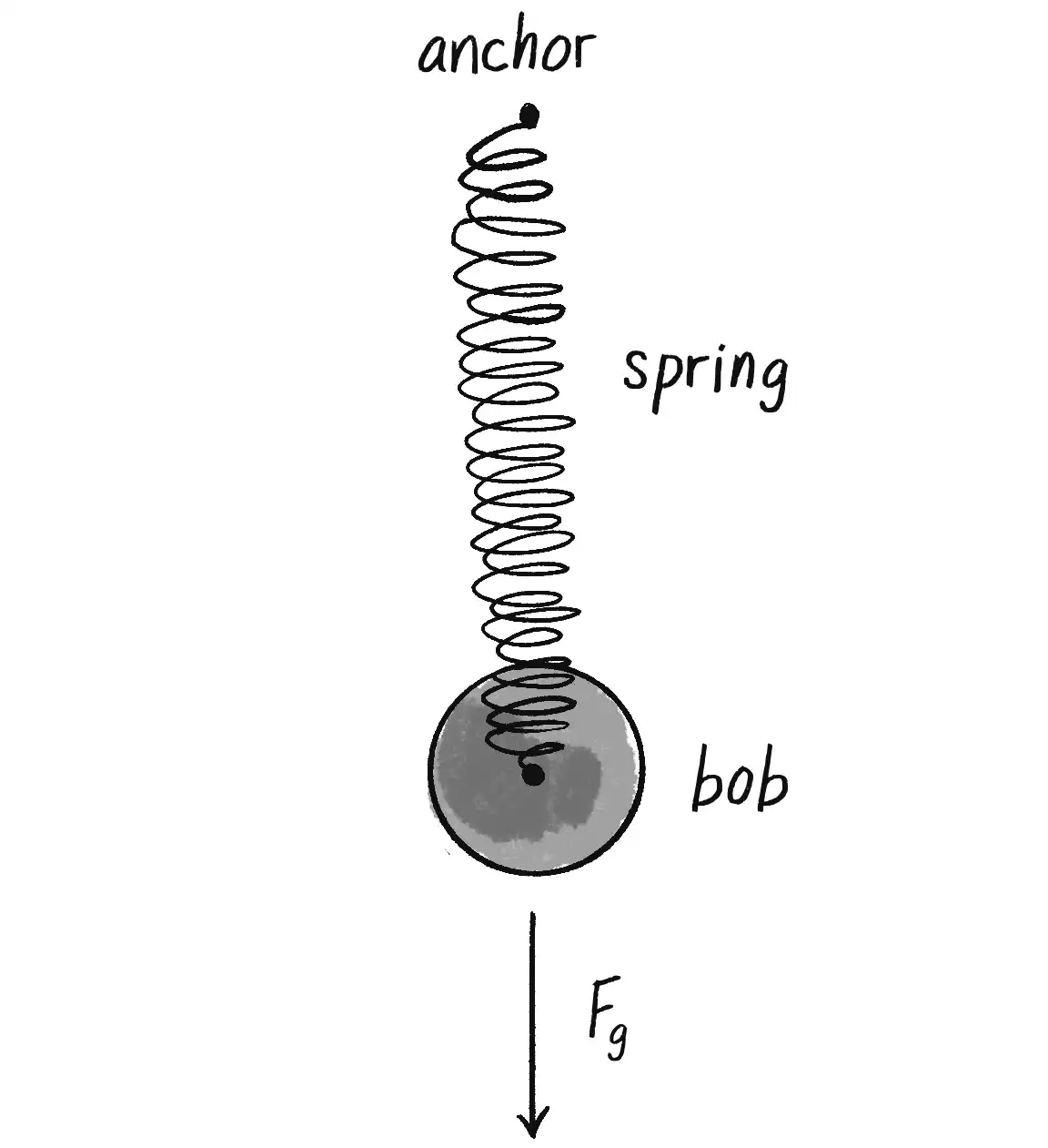
Exploring the mathematics of triangles and waves has been lovely, but perhaps you’re starting to miss Newton’s laws of motion and vectors. After all, the core of this book is about simulating the physics of moving bodies. In “Properties of Oscillation”, I modeled simple harmonic motion by mapping a sine wave to a range of pixels on a canvas. Exercise 3.7 asked you to use this technique to create a simulation of a bob hanging from a spring with the sin() function. That kind of quick-and-dirty, one-line-of-code solution won’t do, however, if what you really want is a bob hanging from a spring that responds to other forces in the environment (wind, gravity, and so on). To achieve a simulation like that, you need to model the force of the spring by using vectors.
I’ll consider a spring to be a connection between a movable bob (or weight) and a fixed anchor point (see Figure 3.14).


The force of the spring is a vector calculated according to Hooke’s law, named for Robert Hooke, a British physicist who developed the formula in 1660. Hooke originally stated the law in Latin: “Ut tensio, sic vis,” or “As the extension, so the force.” Think of it this way:
The force of the spring is directly proportional to the extension of the spring.
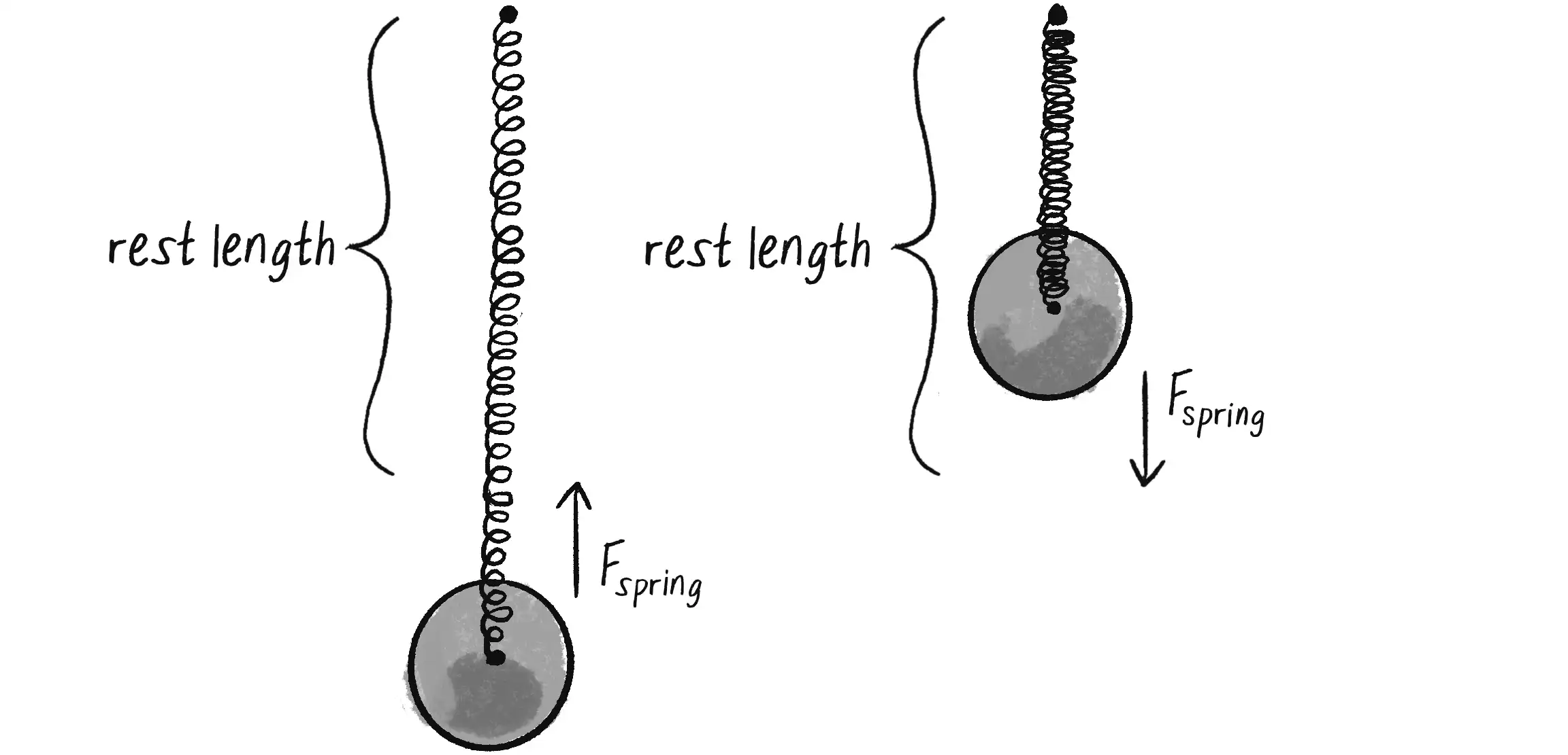
The extension is a measure of how much the spring has been stretched or compressed: as shown in Figure 3.15, it’s the difference between the current length of the spring and the spring’s resting length (its equilibrium state). Hooke’s law therefore says that if you pull on the bob a lot, the spring’s force will be strong, whereas if you pull on the bob a little, the force will be weak.
Mathematically, the law is stated as follows:
Here k is the spring constant. Its value scales the force, setting how elastic or rigid the spring is. Meanwhile, x is the extension, the current length minus the rest length.
Now remember, force is a vector, so you need to calculate both magnitude and direction. For the code, I’ll start with the following three variables—two vectors for the anchor and bob positions, and one rest length:
let anchor = createVector(0, 0);
let bob = createVector(0, 120);
let restLength = 100;
Pick arbitrary values for the positions and rest length.
I’ll then use Hooke’s law to calculate the magnitude of the force. For that, I need k and x. Calculating k is easy; it’s just a constant, so I’ll make something up:
let k = 0.1;
Finding x is perhaps a bit more difficult. I need to know the difference between the current length and the rest length. The rest length is defined as the variable restLength. What’s the current length? The distance between the anchor and the bob. And how can I calculate that distance? How about the magnitude of a vector that points from the anchor to the bob? (Note that this is exactly the same process I employed to find the distance between objects for the purposes of calculating gravitational attraction in Chapter 2.)
let dir = p5.Vector.sub(bob, anchor);
A vector pointing from the anchor to the bob gives you the current length of the spring.
let currentLength = dir.mag();
let x = currentLength - restLength;
Now that I’ve sorted out the elements necessary for the magnitude of the force (–kx), I need to figure out the direction, a unit vector pointing in the direction of the force. The good news is that I already have this vector. Right? Just a moment ago I asked the question, “How can I calculate that distance?” and I answered, “How about the magnitude of a vector that points from the anchor to the bob?” Well, that vector describes the direction of the force!
Figure 3.16 shows that if you stretch the spring beyond its rest length, a force should pull it back toward the anchor. And if the spring shrinks below its rest length, the force should push it away from the anchor. The Hooke’s law formula accounts for this reversal of direction with the –1.

All I need to do now is set the magnitude of the vector used for the distance calculation. Let’s take a look at the code and rename that vector variable force:
let k = 0.1;
let force = p5.Vector.sub(bob, anchor);
let currentLength = force.mag();
let x = currentLength - restLength;
The magnitude of the spring force according to Hooke’s law
force.setMag(-1 * k * x);
Put it together: direction and magnitude!
Now that I have the algorithm for computing the spring force, the question remains: What OOP structure should I use? This is one of those situations that has no one correct answer. Several possibilities exist, and the one I choose depends on my goals and personal coding style.
Since I’ve been working all along with a Mover class, I’ll stick with this same framework. I’ll think of the Mover class as the spring’s bob. The bob needs position, velocity, and acceleration vectors to move about the canvas. Perfect—I have those already! And perhaps the bob experiences a gravity force via the applyForce() method. This leaves just one more step, applying the spring force:
let bob;
function setup() {
bob = new Bob();
}
function draw() {
  let gravity = createVector(0, 1);
  bob.applyForce(gravity);
Chapter 2’s make-up-a-gravity force
  let springForce = _______________????
  bob.applyForce(springForce);
Calculate and apply a spring force!
  bob.update();
  bob.show();
The standard update() and show() methods
}
One option would be to write all the spring-force code in the main draw() loop. But thinking ahead to when you might have multiple bob and spring connections, it would be wise to create an additional class, a Spring class. As shown in Figure 3.17, the Bob class keeps track of the bob’s movements; the Spring class keeps track of the spring’s anchor position and its rest length, and calculates the spring force on the bob.

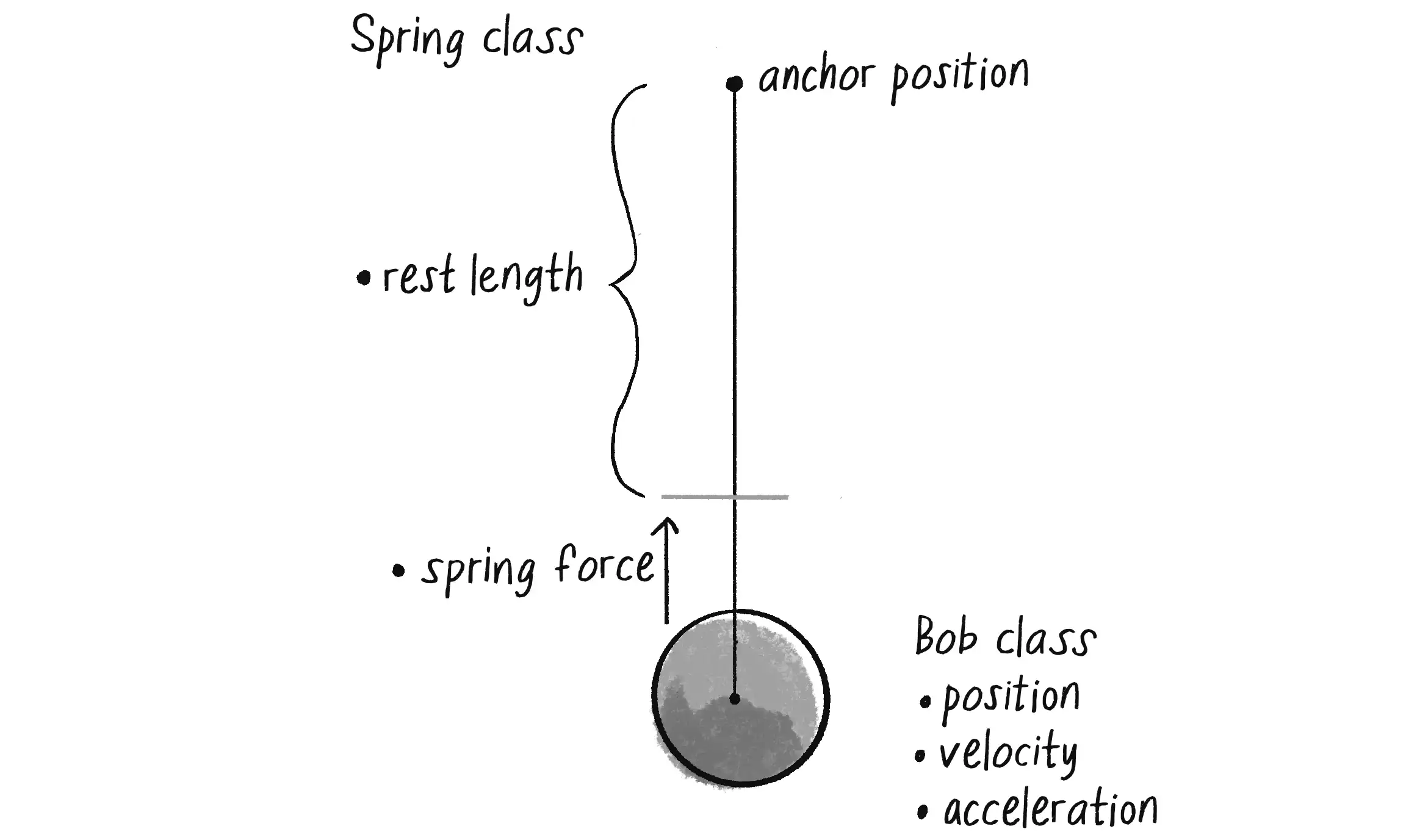
Spring class has anchor and rest length; the Bob class has position, velocity, and acceleration.This allows me to write a lovely sketch as follows:
let bob;
let spring;
Add a Spring object.
function setup() {
bob = new Bob();
spring = new Spring();
}
function draw() {
let gravity = createVector(0, 1);
bob.applyForce(gravity);
spring.connect(bob);
This new method in the Spring class will take care of computing the force of the spring on the bob.
bob.update();
bob.show();
spring.show();
}
Think about how this compares to my first stab at gravitational attraction in Example 2.6, when I had separate Mover and Attractor classes. There, I wrote something like this:
let force = attractor.attract(mover);
mover.applyForce(force);
The analogous situation with a spring might have been as follows:
let force = spring.connect(bob);
bob.applyForce(force);
Instead, in this example I have the following:
spring.connect(bob);
What gives? Why don’t I need to call applyForce() on the bob? The answer, of course, is that I do need to call applyForce() on the bob. It’s just that instead of doing it in draw(), I’m demonstrating that a perfectly reasonable (and sometimes preferable) alternative is to ask the connect() method to call applyForce() on the bob internally:
connect(bob) {
let force = some fancy calculations
bob.applyForce(force);
The connect() method takes care of calling applyForce() and therefore doesn’t have to return a vector to the calling area.
}
Why do it one way with the Attractor class and another way with the Spring class? When I first discussed forces, showing all the forces being applied in the draw() loop was a clearer way to help you learn about force accumulation. Now that you’re more comfortable, perhaps it’s simpler to embed some of the details inside the objects themselves.
Let’s take a look at the rest of the elements in the Spring class.
Example 3.10: A Spring Connection
class Spring {
constructor(x, y, length) {
The constructor initializes the anchor point and rest length.
this.anchor = createVector(x, y);
The spring’s anchor position
    this.restLength = length;
    this.k = 0.2;
Rest length and spring constant variables
}
connect(bob) {
Calculate the spring force as an implementation of Hooke’s law.
let force = p5.Vector.sub(bob.position, this.anchor);
Get a vector pointing from the anchor to the bob position.
    let currentLength = force.mag();
    let stretch = currentLength - this.restLength;
Calculate the displacement between distance and rest length. I’ll use the variable name stretch instead of x to be more descriptive.
force.setMag(-1 * this.k * stretch);
Direction and magnitude together!
bob.applyForce(force);
Call applyForce() right here!
}
  show() {
    fill(127);
    circle(this.anchor.x, this.anchor.y, 10);
  }
Draw the anchor.
  showLine(bob) {
    stroke(0);
Draw the spring connection between the bob position and the anchor.
    line(bob.position.x, bob.position.y, this.anchor.x, this.anchor.y);
  }
}
The complete code for this example is available on the book’s website and incorporates two additional features: (1) the Bob class includes methods for mouse interactivity, allowing you to drag the bob around the window, and (2) the Spring class includes a method to constrain the connection’s length between a minimum and a maximum value.
Exercise 3.13
Before running to see the example online, take a look at this constrainLength method and see if you can fill in the blanks:
constrainLength(bob, minlen, maxlen) {
let direction = p5.Vector.sub(bob.position, this.anchor);
A vector pointing from the bob to the anchor
let length = direction.mag();
if (length < minlen) {
Is it too short?
direction.setMag(minlen);
bob.position = p5.Vector.add(this.anchor, direction);
Keep the position within the constraint.
bob.velocity.mult(0);
} else if (length > maxlen) {
Is it too long?
direction.setMag(maxlen);
bob.position = p5.Vector.add(this.anchor, direction);
Keep the position within the constraint.
bob.velocity.mult(0);
}
}
Exercise 3.14
Create a system of multiple bobs and spring connections. How about connecting a bob to another bob with no fixed anchor?
The Pendulum


You might have noticed that in Example 3.10’s spring code, I never once used sine or cosine. Before you write off all this trigonometry stuff as a tangent, however, allow me to show an example of how it all fits together. Imagine a bob hanging from an anchor connected by a spring with a fully rigid connection that can be neither compressed nor extended. This idealized scenario describes a pendulum and provides an excellent opportunity to practice combining all that you’ve learned about forces and trigonometry.
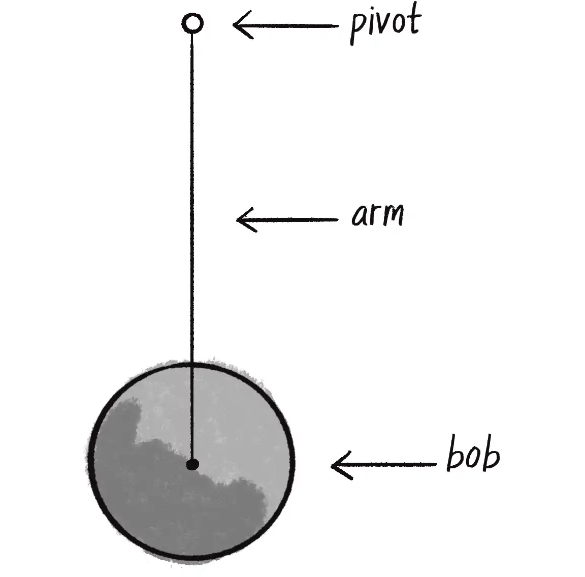
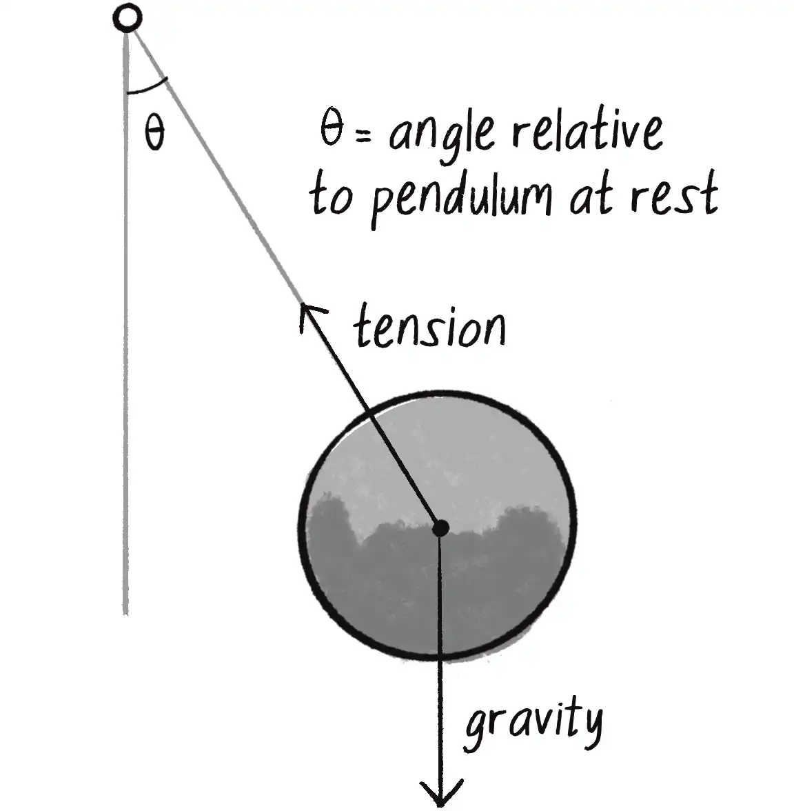
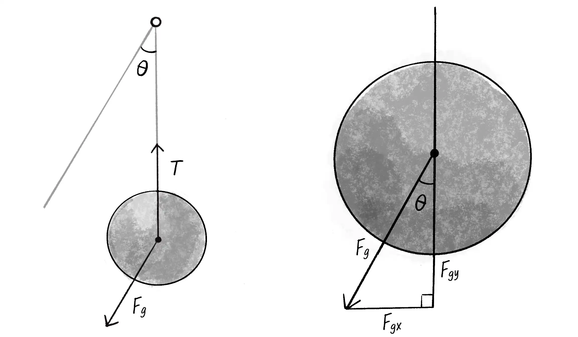
A pendulum is a bob suspended by an arm from a pivot (previously called the anchor in the spring). When the pendulum is at rest, it hangs straight down, as in Figure 3.18. If you lift up the pendulum at an angle from its resting state and then release it, however, it starts to swing back and forth, tracing the shape of an arc. A real-world pendulum would live in a 3D space, but I’m going to look at a simpler scenario: a pendulum in the 2D space of a p5.js canvas. Figure 3.19 shows the pendulum in a nonresting position and adds the forces at play: gravity and tension.
When the pendulum swings, its arm and bob are essentially rotating around the fixed point of the pivot. If no arm connected the bob and the pivot, the bob would simply fall to the ground under the influence of gravity. Obviously, that isn’t what happens. Instead, the fixed length of the arm creates the second force—tension. However, I’m not going to work with this scenario according to these forces, at least not in the way I approached the spring scenario.

Instead of using linear acceleration and velocity, I’m going to describe the motion of the pendulum in terms of angular acceleration and angular velocity, which refer to the change of the arm’s angle relative to the pendulum’s resting position. I should first warn you, especially if you’re a seasoned physicist, that I’m going to conveniently ignore several important concepts here: conservation of energy, momentum, centripetal force, and more. This isn’t intended to be a comprehensive description of pendulum physics. My goal is to offer you an opportunity to practice your new skills in trigonometry and further explore the relationship between forces and angles through a concrete example.
To calculate the pendulum’s angular acceleration, I’m going to use Newton’s second law of motion but with a little trigonometric twist. Take a look at Figure 3.19 and tilt your head so that the pendulum’s arm becomes the vertical axis. The force of gravity suddenly points askew, a little to the left—it’s at an angle with respect to your tilted head. If this is starting to hurt your neck, don’t worry. I’ll redraw the tilted figure and relabel the forces for gravity and for tension (Figure 3.20, left).
Let’s now take the force of gravity and divide its vector into x- and y-components, with the arm as the new y-axis. These components form a right triangle, with the force of gravity as the hypotenuse (Figure 3.20, right). I’ll call them and , but what do these components mean? Well, the component represents the force that’s opposite to , the tension force. Remember, the tension force is what keeps the bob from falling off.
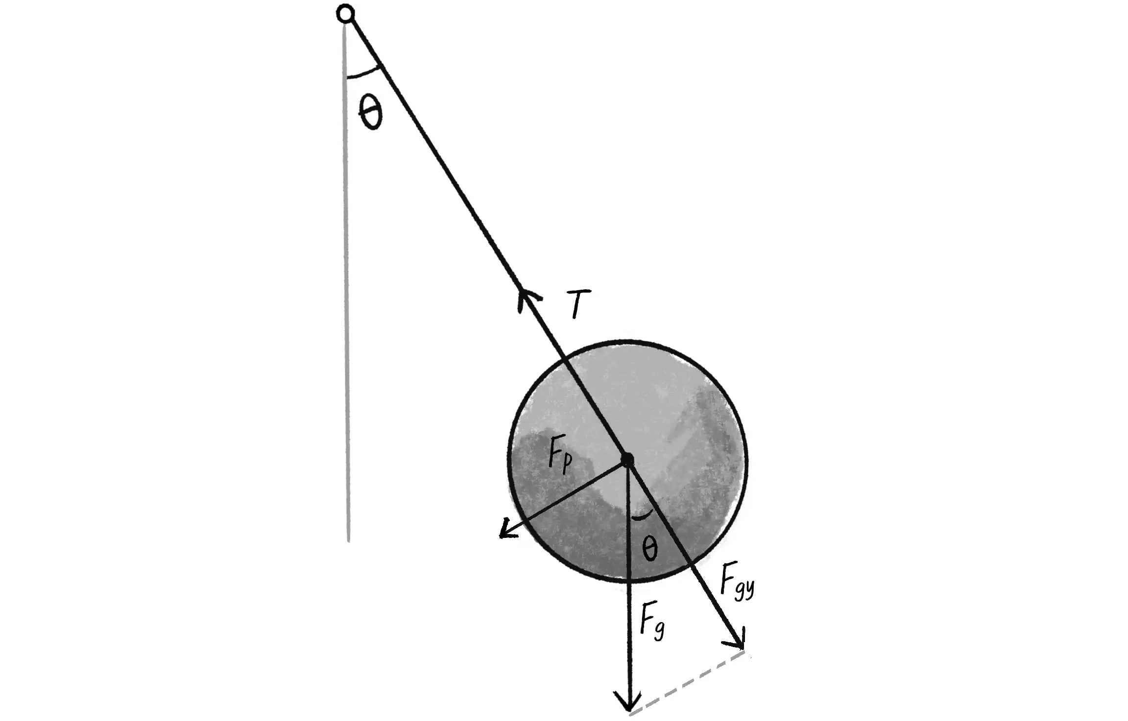
The other component, , is perpendicular to the arm of the pendulum, and it’s the force I’ve been looking for all along! It causes the pendulum to rotate. As the pendulum swings, the y-axis (the arm) will always be perpendicular to the direction of motion. Therefore, I can ignore the tension and forces and focus on , which is the net force in the direction of motion. And because this force is part of a right triangle, I can calculate it with . . . you guessed it, trigonometry!

The key here is that the top angle of the right triangle is the same as the angle between the pendulum’s arm and its resting position. Just as I demonstrated in the discussion of polar coordinates, the sine and cosine functions allow me to separate out the components of the gravity force (the hypotenuse) according to this angle. For , I need to use sine:
Solving for , I get this:
I’ll now rename this force for force of the pendulum. In Figure 3.21, I’ve restored the diagram to its original orientation and relabeled the components. I’ve also moved the starting point of from the bottom of the right triangle to the bob’s center, to clarify how this force moves the bob.
There it is. The net force of the pendulum that causes the rotation is calculated as follows:

Lest you forget, however, my goal is to determine the angular acceleration of the pendulum. Once I have that, I’ll be able to apply the rules of motion to find a new angle for each frame of the animation:
The good news is that Newton’s second law establishes a relationship between force and acceleration—namely, , or . So if the force of the pendulum is equal to the force of gravity times the sine of the angle, then I have this:
This is a good time for a reminder that the context here is creative coding and not pure physics. Yes, the acceleration due to gravity on Earth is 9.8 meters per second squared. But this number isn’t relevant in our world of pixels. Instead, I’ll use an arbitrary constant (called gravity) as a variable that scales the acceleration (incidentally, angular acceleration is usually written as so as to distinguish it from linear acceleration ):
Before I put everything together, there’s another detail I neglected to mention. Or really, lots of little details. Think about the pendulum arm for a moment. Is it a metal rod? A string? A rubber band? How is it attached to the pivot point? How long is it? What’s its mass? Is it a windy day? I could continue to ask a lot of questions that would affect the simulation. I choose to live, however, in a fantasy world, one where the pendulum’s arm is an idealized rod that never bends and where the mass of the bob is concentrated in a single, infinitesimally small point.
Even though I prefer not to worry myself with all these questions, a critical piece is still missing, related to the calculation of angular acceleration. To keep the derivation of the pendulum’s angular acceleration simple, I assumed that the length of the pendulum’s arm is 1. In reality, however, the length of the pendulum’s arm affects the acceleration of the pendulum because of the concepts of torque and moment of inertia.
Torque (or ) is a measure of the rotational force acting on an object. In the case of a pendulum, torque is proportional to both the mass of the bob and the length of the arm (). The moment of inertia (or ) of a pendulum is a measure of the amount of difficulty in rotating the pendulum around the pivot point. It’s proportional to the mass of the bob and the square of the length of the arm ().
Remember Newton’s second law, ? Well, it has a rotational counterpart, . By rearranging the equation to solve for the angular acceleration , I get . Simplifying further, this becomes or . The angular acceleration doesn’t depend on the pendulum’s mass!
This is just like Galileo’s Leaning Tower of Pisa experiment demonstrating linear acceleration, where different objects fell at the same rate, regardless of their mass. Here, once again, the mass of a bob doesn’t influence its angular acceleration—only the length of its arm does. Thus, the final formula becomes this:
Amazing! In the end, the formula is so simple that you might be wondering why I bothered going through the explanation at all. I mean, learning is great, but I could have easily just said, “Hey, the angular acceleration of a pendulum is a constant times the sine of the angle divided by the length of the arm.” That would be missing the point. The purpose of this book isn’t to learn how pendulums swing or gravity works. The point is to think creatively about how shapes can move around a screen in a computationally based graphics system. The pendulum is just a case study. If you can understand the approach to programming a pendulum, you can apply the same techniques to other scenarios, no matter how you choose to design your p5.js canvas world.
Now, I’m not finished yet. I may be happy with my simple, elegant formula for angular acceleration, but I still have to apply it in code. This is an excellent opportunity to practice some OOP skills and create a Pendulum class. First, think about all the properties of a pendulum that I’ve mentioned:
- Arm length
- Angle
- Angular velocity
- Angular acceleration
The Pendulum class needs all these properties too:
class Pendulum {
constructor() {
this.r = ????;
Length of arm
this.angle = ????;
Pendulum arm angle
this.angleVelocity = ????;
Angular velocity
this.angleAcceleration = ????;
Angular acceleration
}
Next, I need to write an update() method to update the pendulum’s angle according to the formula:
update() {
let gravity = 0.4;
An arbitrary constant
this.angleAcceleration = -1 * gravity * sin(this.angle) / this.r;
Calculate acceleration according to the formula.
this.angleVelocity += this.angleAcceleration;
Increment the velocity.
this.angle += this.angleVelocity;
Increment the angle.
}
Note that the acceleration calculation now includes a multiplication by –1. When the pendulum is to the right of its resting position, the angle is positive, and so the sine of the angle is also positive. However, gravity should pull the bob back toward the resting position. Conversely, when the pendulum is to the left of its resting position, the angle is negative, and so its sine is negative too. In this case, the pulling force should be positive. Multiplying by –1 is necessary in both scenarios.
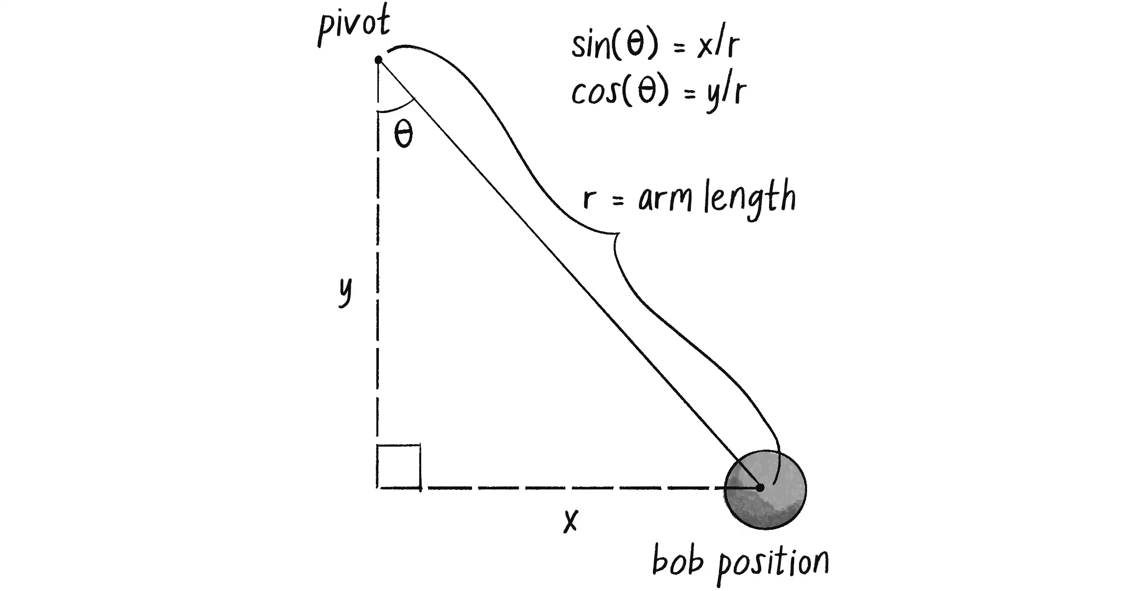
Next, I need a show() method to draw the pendulum on the canvas. But where exactly should I draw it? How do I calculate the x- and y-coordinates (Cartesian!) for both the pendulum’s pivot point (let’s call it pivot) and bob position (let’s call it bob)? This may be getting a little tiresome, but the answer, yet again, is trigonometry, as shown in Figure 3.22.

First, I’ll need to add a this.pivot property to the constructor to specify where to draw the pendulum on the canvas:
this.pivot = createVector(100, 10);
I know the bob should be a set distance away from the pivot, as determined by the arm length. That’s my variable r, which I’ll set now:
this.r = 125;
I also know the bob’s current angle relative to the pivot: it’s stored in the variable angle. Between the arm length and the angle, what I have is a polar coordinate for the bob: . What I really need is a Cartesian coordinate, but luckily I already know how to use sine and cosine to convert from polar to Cartesian. And so:
this.bob = createVector(r * sin(this.angle), r * cos(this.angle));
Notice that I’m using sin(this.angle) for the x value and cos(this.angle) for the y. This is the opposite of what I showed you in “Polar vs. Cartesian Coordinates”. The reason is that I’m now looking for the top angle of a right triangle pointing down, as depicted in Figure 3.21. This angle lives between the y-axis and the hypotenuse, instead of between the x-axis and the hypotenuse, as you saw earlier in Figure 3.9.
Right now, the value of this.bob is assuming that the pivot is at point (0, 0). To get the bob’s position relative to wherever the pivot actually happens to be, I can just add pivot to the bob vector:
this.bob.add(this.pivot);
Now all that remains is the little matter of drawing a line and a circle (you should be more creative, of course):
stroke(0);
fill(127);
line(this.pivot.x, this.pivot.y, this.bob.x, this.bob.y);
circle(this.bob.x, this.bob.y, 16);
Finally, a real-world pendulum is going to experience a certain amount of friction (at the pivot point) and air resistance. As it stands, the pendulum would swing forever with the given code. To make it more realistic, I can slow the pendulum with a damping trick. I say trick because rather than model the resistance forces with some degree of accuracy (as I did in Chapter 2), I can achieve a similar result simply by reducing the angular velocity by an arbitrary amount during each cycle. The following code reduces the velocity by 1 percent (or multiplies it by 0.99) for each frame of animation:
this.angleVelocity *= 0.99;
Putting everything together, I have the following example (with the pendulum beginning at a 45-degree angle).
Example 3.11: Swinging Pendulum
let pendulum;
function setup() {
createCanvas(640, 240);
pendulum = new Pendulum(width / 2, 0, 175);
Make a new Pendulum object with an origin position and arm length.
}
function draw() {
background(255);
pendulum.update();
pendulum.show();
}
class Pendulum {
constructor(x, y, r) {
    this.pivot = createVector(x, y); // Position of pivot
    this.bob = createVector(0, 0);   // Position of bob
    this.r = r;                      // Length of arm
    this.angle = PI / 4;             // Pendulum arm angle
    this.angleVelocity = 0;          // Angle velocity
    this.angleAcceleration = 0;      // Angle acceleration
    this.damping = 0.99;             // Arbitrary damping
    this.ballr = 24;                 // Arbitrary bob radius
Many, many variables keep track of the pendulum’s various properties.
}
update() {
let gravity = 0.4;
this.angleAcceleration = (-1 * gravity / this.r) * sin(this.angle);
Formula for angular acceleration
    this.angleVelocity += this.angleAcceleration;
    this.angle += this.angleVelocity;
Standard angular motion algorithm
this.angleVelocity *= this.damping;
Apply some damping.
}
show() {
    this.bob.set(this.r * sin(this.angle), this.r * cos(this.angle));
    this.bob.add(this.pivot);
Apply polar-to-Cartesian conversion. Instead of creating a new vector each time, I’ll use set() to update the bob’s position.
    stroke(0);
    line(this.pivot.x, this.pivot.y, this.bob.x, this.bob.y);
The arm
    fill(127);
    circle(this.bob.x, this.bob.y, this.ballr * 2);
The bob
}
}
On the book’s website, this example has additional code to allow the user to grab the pendulum and swing it with the mouse.
Exercise 3.15
String together a series of pendulums so that the bob of one is the pivot point of another. Note that doing this may produce intriguing results but will be wildly inaccurate physically. Simulating an actual double pendulum requires sophisticated equations. You can read about them in the Wolfram Research article on double pendulums or watch my video on coding a double pendulum.
Exercise 3.16

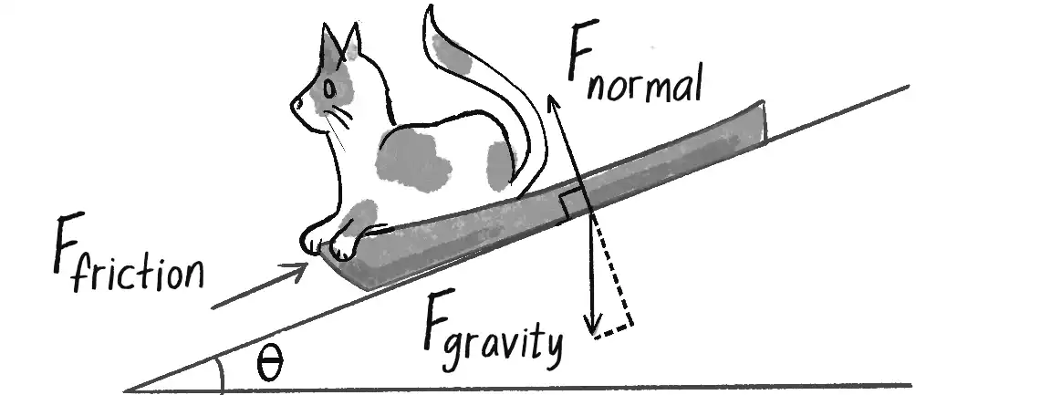
Using trigonometry, how do you calculate the magnitude of the normal force depicted here (the force perpendicular to the incline on which the sled rests)? You can consider the magnitude of to be a known constant. Look for a right triangle to help get you started. After all, the normal force is equal and opposite to a component of the force of gravity. If it helps to draw over the diagram and make more right triangles, go for it!
Exercise 3.17
Create a simulation of a box sliding down an incline with friction. Note that the magnitude of the friction force is proportional to the normal force, as discussed in the previous exercise.
The Ecosystem Project
Take one of your creatures and incorporate oscillation into its motion. You can use the Oscillator class from Example 3.7 as a model. The Oscillator object, however, oscillates around a single point (the middle of the window). Try oscillating around a moving point.
In other words, design a creature that moves around the screen according to position, velocity, and acceleration. But that creature isn’t just a static shape; it’s an oscillating body. Consider tying the speed of oscillation to the speed of motion. Think of a butterfly’s flapping wings or the legs of an insect. Can you make it appear as though the creature’s internal mechanics (oscillation) drive its locomotion? See the book’s website for an additional example combining attraction from Chapter 2 with oscillation.